Week 4.1 - Genetic Algorithm

Aim : Optimization of Stalagmite Function Using Genetic Algorithm

Objective :

• Find the global maxima
• - Plotting the graph for all 3 studies for function maximum vs no. of iterations

Theory :

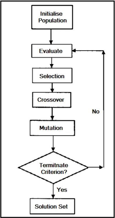
Genetic Algorithms (GAs) are adaptive heuristic search algorithms that belong to the larger part of evolutionary algorithms. Genetic algorithms are based on the ideas of natural selection and genetics. These are intelligent exploitation of random search provided with historical data to direct the search into the region of better performance in solution space. They are commonly used to generate high-quality solutions for optimization problems and search problems.

Genetic algorithms simulate the process of natural selection which means those species who can adapt to changes in their environment are able to survive and reproduce and go to next generation. In simple words, they simulate "survival of the fittest" among individual of consecutive generation for solving a problem. Each generation consist of a population of individuals and each individual represents a point in search space and possible solution. Each individual is represented as a string of character/integer/float/bits. This string is analogous to the Chromosome.

Genetic algorithms are based on an analogy with genetic structure and behavior of chromosome of the population. Following is the foundation of GAs based on this analogy

• Individual in population compete for resources and mate. -
• Those individuals who are successful (fittest) then mate to create more offspring than others
• Genes from "fittest" parent propagate throughout the generation, that is sometimes parents create offspring which is better than either parent.
• Thus each successive generation is more suited for their environment.

Search Space :

The population of individuals are maintained within search space. Each individual represent a solution in search space for given problem. Each individual is coded as a finite length vector (analogous to chromosome) of components. These variable components are analogous tc Genes. Thus a chromosome (individual) is composed of several genes (variable components).

Fitness Score :

A Fitness Score is given to each individual which shows the ability of an individual to "compete". The individual having optimal fitness score (or near optimal) are sought.

Operators of Genetic Algorithms :

Once the initial generation is created, the algorithm evolve the generation using following operators

1. Selection Operator : The idea is to give preference to the individuals with good fitness scores and allow them to pass there genes to the successive generations.
2. Crossover Operator : This represents mating between individuals. Two individuals are selected using selection operator and crossover sites are chosen randomly. Then the genes at these crossover sites are exchanged thus creating a completely new individual
3. Mutation Operator: The key idea is to insert random genes in offspring to maintain the diversity in population to avoid the premature convergence.

Following are the Syntax used for finding the maximum of function using genetic algorithm :

x = ga(fun , nvars) finds a local unconstrained minimum, x, to the objective function, fun. nvars is the dimension (number of design variables) of fun.

x = ga(fun,nvars,A,b,Aeq,beq,lb,ub) defines a set of lower and upper bounds on the design variables, x, so that a solution is found in the range lb 5 x 5 ub. (Set Aeq=0 and beq=1:1 if no linear equalities exist.)

x = ga(fun,nvars,A,b,Aeq,beq,lb,ub,nonlcon,options) minimizes with the default optimization parameters replaced by values in options. (Set nonlcon=0 if no nonlinear constraints exist.) Create options using optimoptions

where,

fun = Objective function

nvars = Numbers of variables

A = Linear inequality constraints

b = Linear inequality constraints

Aeq = Linear equality constraints

beq = Linear equality constraints

lb = Lower bounds

ub = Upper bounds

nonlcon = Nonlinear

constraints options = Optimization options

clear all 
close all 
clc

x=linspace(0,0.6,150);
y=linspace(0,0.6,150);
[xx,yy]=meshgrid(x,y);
num_cases = 50
for p=1:length(x)
for q=1:length(y)
    input_vector(1)=xx(p,q)
    input_vector(2)=yy(p,q)
tic
f(p,q) = stagalmite(input_vector);
end
end
study1_time=toc

%study 1 - statastical behevior
for i = 1:num_cases
    [inputs, fopt(i)] = ga(@stagalmite, 2);
    xopt(i) = inputs(1);
    yopt(i) = inputs(2);
end

figure(1)
subplot(2,1,1)
hold on 
surfc(x,y,f)
shading interp
plot(xopt,yopt,'marker','o','MarkerSize',5,'markerfacecolor','r')
    subplot(2,1,2)
    plot(fopt)
    xlabel('Iterations')
    ylabel('Function minimun')

tic
%study 2 -statastical beheviour - with upper and lower bounds 
for i=1:num_cases
    [inputs,fopt(i)]=ga(@stagalmite,2,[],[],[],[],[0:0],[1:1]);
    xopt(i) = inputs(1);
    yopt(i) - inputs(2);
end
study2_time = toc

figure(2)
subplot(2,1,1)
hold on 
surfc(x,y,f)
shading interp
plot(xopt,yopt,'marker','o','markersize',5,'markerfacecolor','r')
    subplot(2,1,2)
    plot(fopt)
    xlabel('Iterations')
    ylabel('Function minimun')

%study 3 increasing GA interations
options = optimoptions('ga')
options = optimoptions(options,'PopulationSize',170)

tic
for i=1:numcases
    [inputs,fopt(i)] = ga(@stagalmite,2,[],[],[],[],[0:0],[1:1],[],[],options);
    xopt(i)= inputs(1);
    yopt(i)= inputs(2);
end
study3_time = toc

figure(3)
subplot(2,1,1)
hold on 
surfc(x,y,f)
shading interp
plot(xopt,yopt,'marker','o','markersize',5,'markerfacecolor','r')
    subplot(2,1,2)
    plot(fopt)
    xlabel('Iterations')
    ylabel('Function minimun')

STALAGMITE FUNCTION CODE:

function A = stagalmite(input_vector)
x=input_vector(1);
y=input_vector(2);
f1=sin(5.1*pi*x+0.5).^6;
f2=exp((-4*log(2)*((x-0.0667).^2))/0.64);
f3=(sin(5.1*pi*y+0.5)).^6;
f4=exp((-4*log(2))*((y-0.0667).^2)/0.64);
A=-(f1*f2*f3*f4);
end

Code Explanation wth Results :

• First write command clear all, close all, clc.
• Setting up the search space for given problem, considering the variables x and y with linspace command.As x,y both are the one dimensional array with the help of meshgrid command are converting them into two dimensional array and variables are xx,yy.
• We have created the seperate function file for given problem statement and function file name is "stalagmite_shivam". In this we have used the formules(f_x_1,f_x_2,f_x_3,f_x_4) and then multiplied it with each other. Here we use negative sign (-) in functionso as to calculate the global maxima.
• Here we have specified the input vector i.e xx and yy, and they are used to give the inputs to the stalagmite_shivam function.
• We are considering the number of iteration to be 50 i.e - "num_cases = 50" . Tic - Toc command is used to measure the time taken by particular study.

Study 1 (unbound inputs):

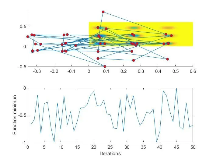
• Now starting with Studyl,here for loop is used and it will run for number of iteration i.e 50. In the for loop we are providing the ga syntax i.e - "ga(estalagmite_shivam,2) " with the stalagmite_shivam function and with two variables. we have also specified the xopt, yopt and fopt.
• We have used surfc command to plot stalagmite_shivam function and below that "shading interp" to hide the grids on the plot.
• Figure is created with figure command and first subplot command, hold on command and plot3 command are used in code to plot the graph of stalagmite_shivam function and graph of unbounded inputs i.e xopt,yopt,fopt together in the figure.
• With the help of second subplot command we have plottted the number of iteration vs function maximum graph in the same figure.
• Xlabel ("Iterations"), ylabel("Maximum value of function"), title("Unbounded Inputs") command used to give graphical representation to graph.
• time was taken by this study is 0.0017.

Study2 (Bounded inputs):

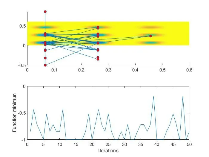
• Now starting with Study2, here for loop is used and it will run for number of iteration i.e 50. Here in this study2 we are giving the limits to genetic algorithms in the form of upper bound and lower bound. Also Linear inequality constraints, Linear inequality constraints are in syntax. Genetic algorithm syntax for this study would be "ga(estalagmite_shivam,2,111:1,111:110;0],[0.6;0.6])".We have also specified the xopt, yopt and fopt.
• We have used surfc command to plot stalagmite_shivam function and below that "shading interp" to hide the grids on the plot.
• Figure is created with figure command and first subplot command, hold on command and plot3 command are used in code to plot the graph of stalagmite_shivam function and graph of unbounded inputs i.e xopt,yopt,fopt together in the figure.
• With the help of second subplot command we have plottted the number of iteration vs function maximum graph in the same figure. -
• Xlabel ("Iterations"), ylabel("Maximum value of function") title ("Bounded Inputs") command used to give graphical representation to graph.
• Time by this study to complete is 614.6815
  
  

Study 3 (Bounded inputs with modified population size)

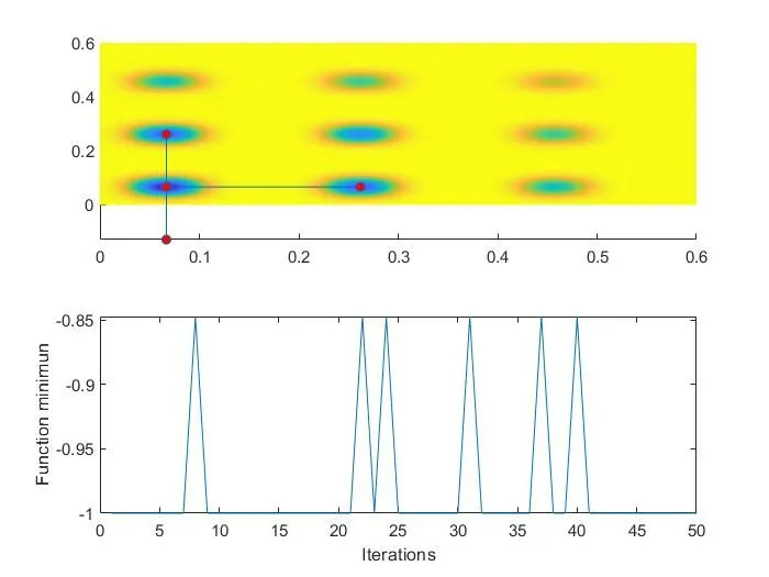
• Now starting with Study3, here for loop is used and it will run for number of iteration i.e 50. In this study we are considering the population size of 300 by using command called optimoptions. Genetic algorithm syntax for this study would be ga(estalagmite_shivam,2,1:a0,0, [0;0],[0.6;0.6],0,aoptions). we have also specified the xopt, yopt and fopt.
• We have used surfc command to plot stalagmite_shivam function and below that "shading interp" to hide the grids on the plot.
• Figure is created with figure command and first subplot command, hold on command and plot3 command are used in code to plot the graph of stalagmite_shivam function and graph of unbounded inputs i.e xopt,yopt,fopt together in the figure.
• With the help of second subplot command we have plottted the number of iteration vs function maximum graph in the same figure. -
• Xlabel ("Iterations"), ylabel("Maximum value of function"), title("Bounded inputs with modified population size")command used to give graphical representation to graph.
• Time by this study to complete 15.7599

ERRORS OCCURED WHILE PROGRAMMING:

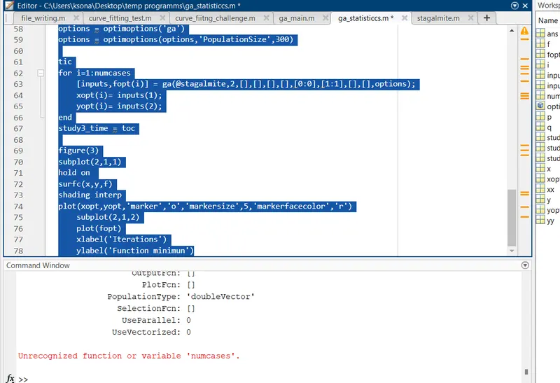
Forgot to use (_) in study 3

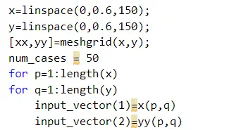
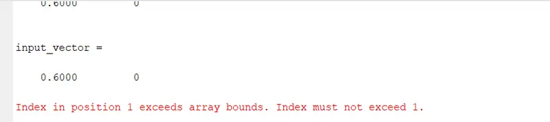
Mistakely only 1 x has been put so the error occured