Week 4.1 - Genetic Algorithm

AIM:

Write a code in MATLAB to optimise the stalagmite function and find the global maxima of the function.

OBJECTIVES OF THE PROJECT:

The requirements are

• Clearly explain the concept of genetic algorithm and the syntax for ga in MATLAB.
• The code gives the same output, even if it is made to run several times.
• Plot graphs for all 3 studies and for F maximum vs no. of iterations.

THEORY:

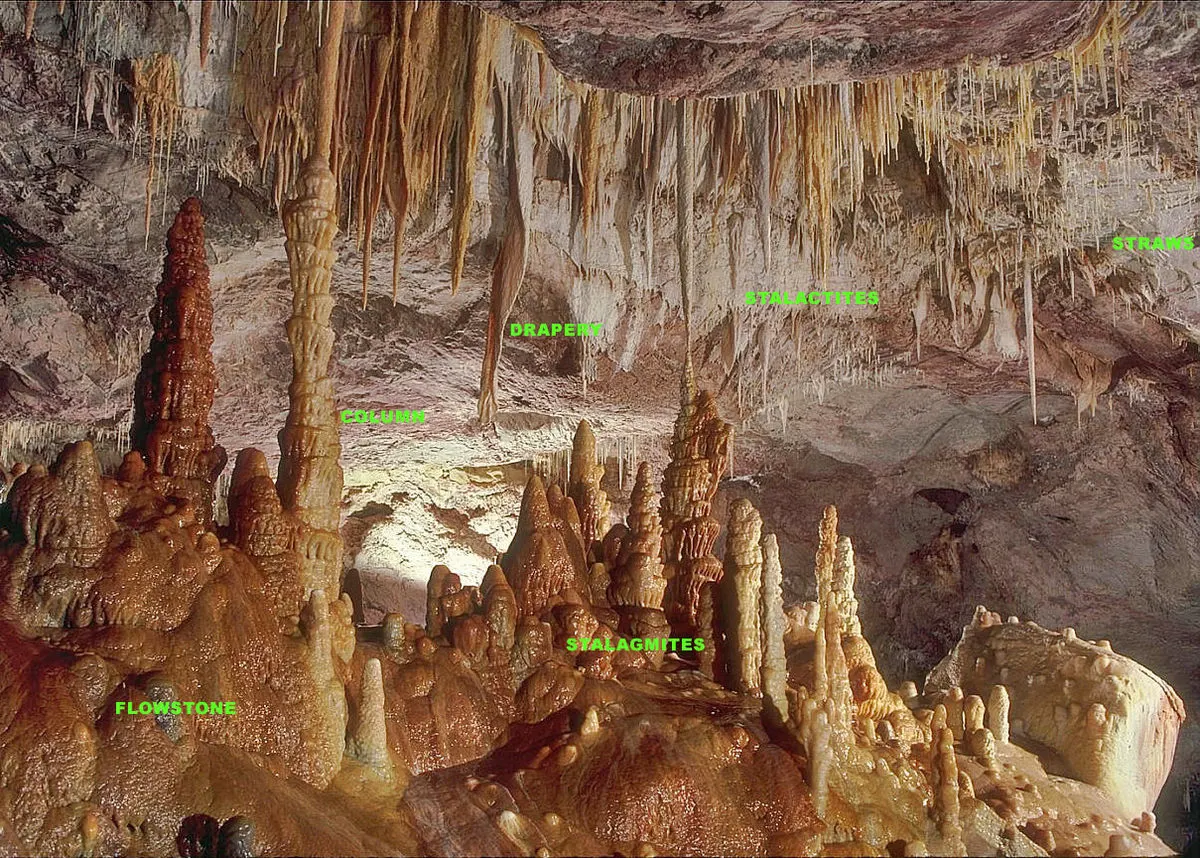
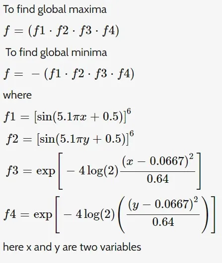
A stalagmite is a type of rock formation that rises from the floor of a cave due to the accumulation of material deposited on the floor from ceiling drippings. Hence the program uses the same logic and the graph is plotted as stalagmite to show the global maxima. The below diagrams show the stalagmite structure and the function formulae which represent a stalagmite:

Genetic Algorithm (ga):

Genetic Algorithm (GA) is a search-based optimization technique based on the principles of Genetics and Natural Selection. It is frequently used to find optimal or near-optimal solutions to difficult problems which otherwise would take a lifetime to solve. It is frequently used to solve optimization problems, in research, and in machine learning. Genetic Algorithms are a method that work based on Darwin's theory of natural selection: The fittest survives, and has a greater chance of breeding and passing forward its genetic information.

The syntax used in the below program are:

• x = ga(fun,nvars,A,b) finds a local minimum x to fun, subject to the linear inequalities A*x ≤ b. ga evaluates the matrix product A*x as if x is transposed (A*x').
• x = ga(fun,nvars,A,b,Aeq,beq,lb,ub,nonlcon,options) minimizes with the default optimization parameters replaced by values in options. (Set nonlcon=[] if no nonlinear constraints exist.) Createoptions using optimoptions.
• [x,fval] = ga(___), for any previous input arguments, also returns fval, the value of the fitness function at x.

PROGRAM:

The codes are done using MATLAB.

1.Code for stalagmite function is as following:

function [f]=stalagmite(input_vector)

x=input_vector(1);
y=input_vector(2);

f1=(sin(5.1*pi*x+0.5))^6;
f2=(sin(5.1*pi*y+0.5))^6;
f3=exp(-4*log(2)*(x-0.0667)^2/0.64);
f4=exp(-4*log(2)*(y-0.0667)^2/0.64);

f=-(f1*f2*f3*f4);
end

2.Code for global maxima is as following:

clear all
close all
clc

%Defining our search space
x = linspace(0,0.6,150);
y = linspace(0,0.6,150);

%Creating a 2Dimensional mesh
[xx yy] = meshgrid(x,y);

num_cases = 50;

%Evaluating the stalgamite function
for i = 1:length(xx)
    for j = 1:length(yy)
        input_vector(1) = xx(i,j);
        input_vector(2) = yy(i,j);
        f(i,j) = stalagmite(input_vector);
    end
end

tic
%Study 1 - Statistical behaviour 
for i = 1:num_cases
  [in1,fopt1(i)] = ga(@stalagmite,2);
  xopt1(i) = in1(1);
  yopt1(i) = in1(2);
end

study1_time = toc

%plotting1
figure(1)
subplot(2,1,1)
hold on
surfc(x,y,-f)
xlabel('x value')
ylabel('y value')
zlabel('z value')
shading interp
plot3(xopt1,yopt1,-fopt1,'marker','o','markersize',5,'markerfacecolor','r')
title('Unbound inputs')
subplot(2,1,2)
plot(-fopt1)
xlabel('Iterations')
ylabel('Function maxima')

tic

%Study 2 - Statistical behaviour - with upper and lower bounds

for i = 1:num_cases
  [in2,fopt2(i)] = ga(@stalagmite,2,[],[],[],[],[0;0],[0.6;0.6]);
  xopt2(i) = in2(1);
  yopt2(i) = in2(2);
end

study2_time = toc

%plotting2
figure(2)
subplot(211)
hold on
surfc(x,y,-f)
shading interp
xlabel('x value')
ylabel('y value')
zlabel('z value')
plot3(xopt2,yopt2,-fopt2,'marker','o','markersize',5,'markerfacecolor','r')
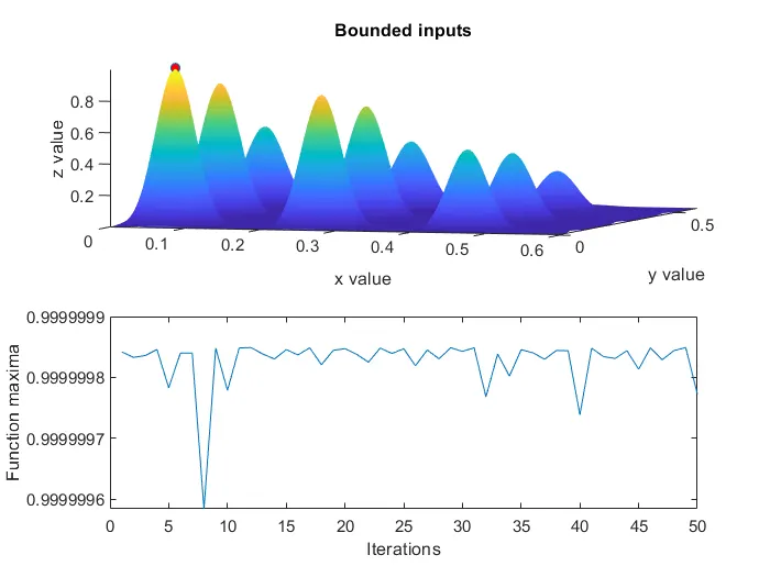
title('Bounded inputs')
subplot(212)
plot(-fopt2)
xlabel('Iterations')
ylabel('Function maxima')

tic

%Study 3 - Increasing ga iteration
options = optimoptions('ga','populationsize',170);

for i = 1:num_cases
  [in3,fopt3(i)] = ga(@stalagmite,2,[],[],[],[],[0;0],[0.6;0.6],[],[],options);
  xopt3(i) = in3(1);
  yopt3(i) = in3(2);
end

study3_time = toc

%plotting3
figure(3)
subplot(211)
hold on
surfc(x,y,-f)
shading interp
xlabel('x value')
ylabel('y value')
zlabel('z value')
plot3(xopt3,yopt3,-fopt3,'marker','o','markersize',5,'markerfacecolor','r')
title('Bounded inputs')
subplot(212)
plot(-fopt3)
xlabel('Iterations')
ylabel('Function maxima')

EXPLANATION OF THE CODE:

The stalagmite function code is according to the formulaes mentioned in the theory.

In the ga statistics program

• Initially a stalagmite is generated by calling the stalagmite function.
• The Study time of each study is calculated using the tic toc
• In Study 1, the statistical behaviour of Genetic Algorithm, a loop is started from 1 to the length of num_cases using the variable i. Calling the genetic algorithm solver by passing the function to solve the stalagmite function with two number of variables. Inputs is the array to store the optimum values if the variables of the stalagmite function as selected. fopt1 is the array to store the optimum values of the stalagmite function for all the values of x and y. In1 and fopt1 are the outputs of the GA. Then saving the value of x selected by GA in the array xopt1 for every iteration of the for loop. And saving the value of y selected by GA in the array yopt1 for every iteration of the for loop.
• In the plotting, surfc command is used to create a surface plot of the values of stalagmite function stored in the array f. Shading interp command is used to generate a smooth plot. Lastly plot3 is used to create a 3D plot of the variables.
• In Study 2, Statistical behaviour - with upper and lower bounds, various inputs are given to the stalagmite function during the function call for simplified analysis. Then the same procedure as Study1 is followed to generate the plot.
• In Study 3, the statistical behaviour of GA by increasing the number of iterations. the optimoptions function is used to return default options to the ga solver. Providing the default options of the ga solver with named parameter Population Size with a value of 170. Then the same procedure as Study1 is followed to generate the plot.

OUTPUT:

Figure 1: Here, as the curve is unbound Random values are generated between 0 & 1.

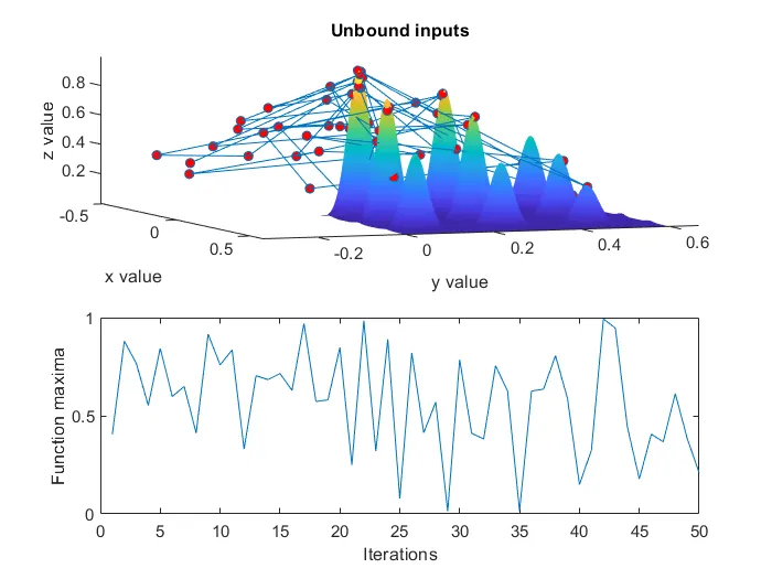
Figure 2: Due to the given constraints in the function calling, the vale\ues becomes bound between 0.85 and 1. A narrowed output is seen and the randomness is decreased.

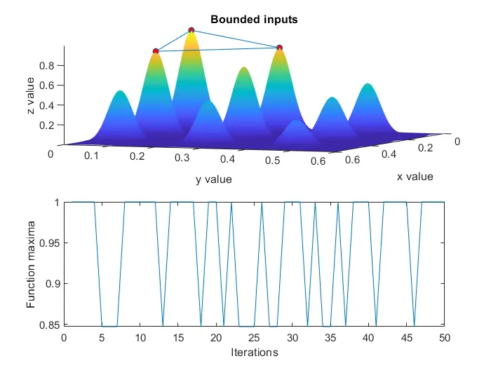
Figure 3:Here the global maxima obtained is accurate and narrowed down to 0.9999996.

CONCLUSION:

The above experiment was completed successfully. The codes and their respective outputs are attached above.