Week 3 - Solving second order ODEs

AIM:

Write a program in MATLAB that will simulate the pendulum motion, using second order ordinary differential equation (ODE).

OBJECTIVES OF THE PROJECT:

The requirements are

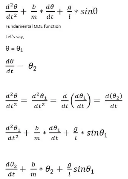
• Solves the following ODE which represents the equation of motion of a simple pendulum with damping.
• Code should show position of the pendulum as a function of time.

THEORY:

A second order ODE is a differential equation in which the highest power of the derivative is 2.

The second order ODE have a huge significance in soving various complex eqautions in mathematics. Here, a pendulum of mass 'm' and length 'l' is hanging from a fixed point, is initially released from an angle theta. The pendulum swings back and forth and finally stops due to damping.

The equation is as follows:

The constraints given here are:

• g = gravity in m/s2,
• L = length of the pendulum in m,
• m = mass of the ball in kg,
• b=damping coefficient.
• L=1 metre,
• m=1 kg,
• b=0.05.
• g=9.81 m/s2.
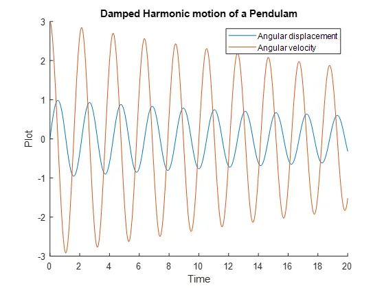
• The motion is between 0-20 sec, for angular displacement=0, angular velocity=3 rad/sec at time t=0.

PROGRAM:

The codes are done using MATLAB.

Function Code of ODE is as following:

function [dtheta_dt] = ode_func(t,theta,b,g,l,m)
    theta1 = theta(1);
    theta2 = theta(2);
    dtheta1_dt = theta2;
    dtheta2_dt = -(b/m)*theta2 - (g/l)*sin(theta1);
    dtheta_dt = [dtheta1_dt; dtheta2_dt];
end

Code Explanation:

The above code solves the above equation along with the assumptions made. It then returns the value to the main program as shown below.

Code of the ODE with Damping Pendulum is as follows:

clear all
close all
clc

%inputs
b = 0.05;
g = 9.81;
l = 1;
m = 1;

%initial conditions
theta_0 = [0;3]; % ; defines column matrix

%time points
t_span = linspace(0,20,400);

%solve ODE
[t, results] = ode45(@(t,theta) ode_func(t,theta,b,g,l,m),t_span,theta_0);

%Plotting
figure(1)
hold on;
plot(t,results(:,1));
plot(t,results(:,2));
title('Damped Harmonic motion of a Pendulam');
legend('Angular displacement', 'Angular velocity');
ylabel('Plot'); xlabel('Time');

%Loop
ct = 1; %counter
for i = 1:length(results(:,1))
    x_start = 0
    y_start = 0
    x_end = 1*sin(results(i,1))
    y_end = -1*cos(results(i,1))
    
    %plotting the animation
    figure(2)
    plot([-1 1], [0 0], 'linewidth', 5); hold on;
    plot([x_start x_end],[y_start y_end],'linewidth',3); hold on;
    
    plot(x_end,y_end,'o','markersize',20,'markerFacecolor','y');
    title('Animation of transient behaviour of a Pendulum');
    axis([-1.5 1.5 -1.5 1]);
    pause(0.01);
    hold off;
    
    M(ct) = getframe(gcf);
    ct = ct+1;
    
end

%Pendulum Animation
movie(M);
videofile = VideoWriter('Pendulum_Animation.avi','uncompressed avi');
open(videofile);
writeVideo(videofile,M);
close(videofile);

Code Explanation:

The above first takes the inputs of various variables and using the equations implemented using formulaes, the various positions of Pendlum is plotted. Each frame of the Pendulum is captured and then combined to form an animation of Damping pendulum.

OUTPUT:

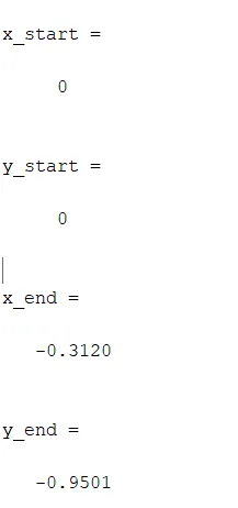
The end results are:

The below figure shows the graph

The animated video clip is obtained as the output for the above code. The video can be viewed by clicking the mentioned link: https://youtu.be/wStz6NO8lC8

CONCLUSION:

The ODE was solved successfully as per the given data and requirements and the animated video of damping pendulum is attached to the link above.