Project 1 - Parsing NASA thermodynamic data
AIM:
Write a function that extracts the 14 co-efficients and calculates the enthalpy, entropy and specific heats for all the species in the data file. You will be reading this file NASA thermodynamic data.
OBJECTIVES OF THE PROJECT:
The requirements are
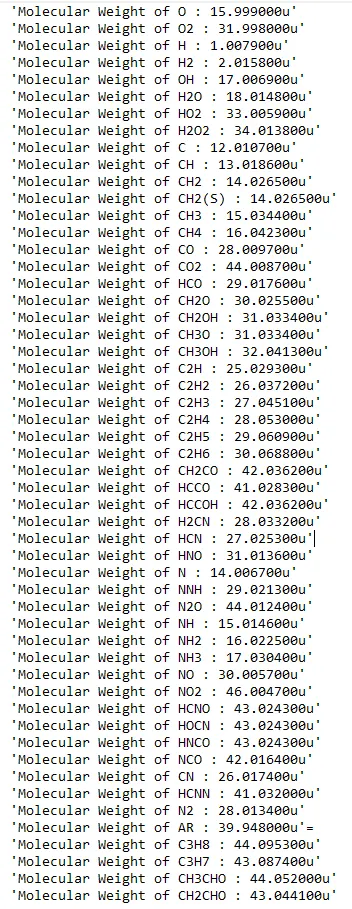
- Calculate the molecular weight of each species and display it in the command window.
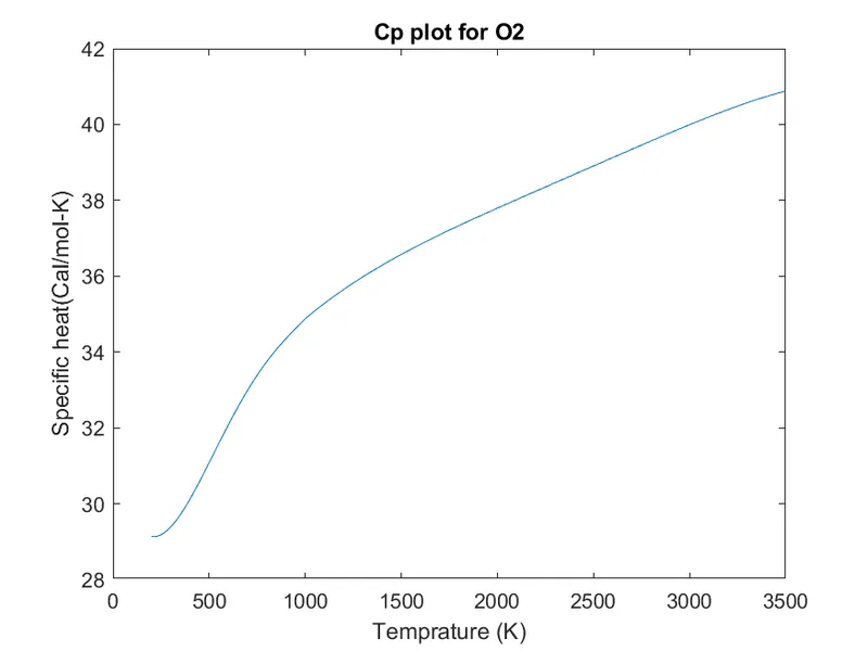
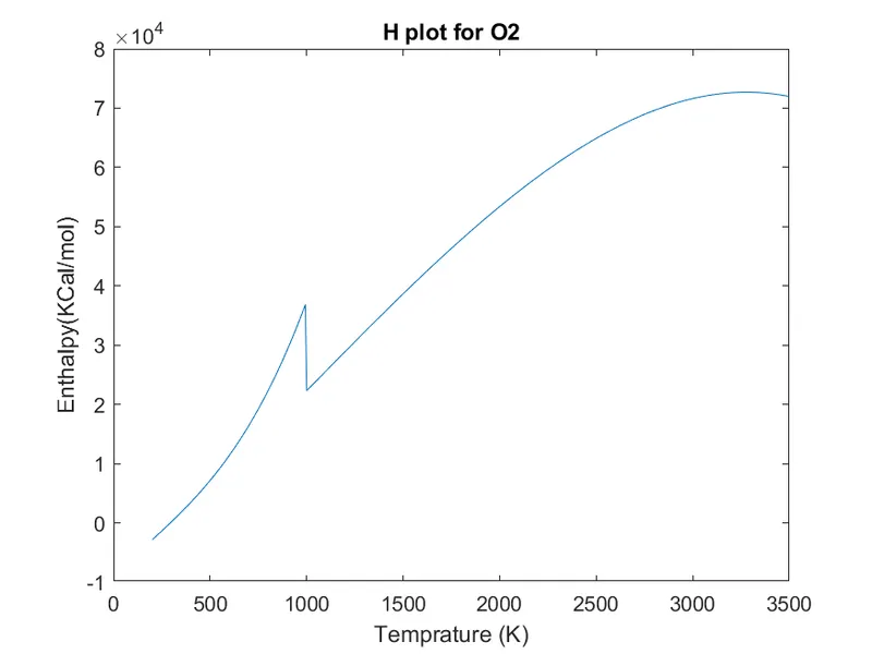
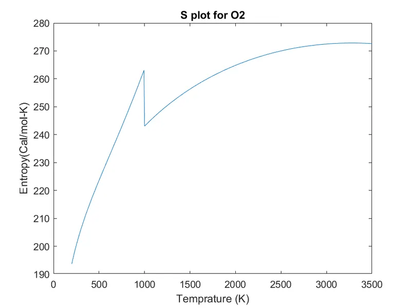
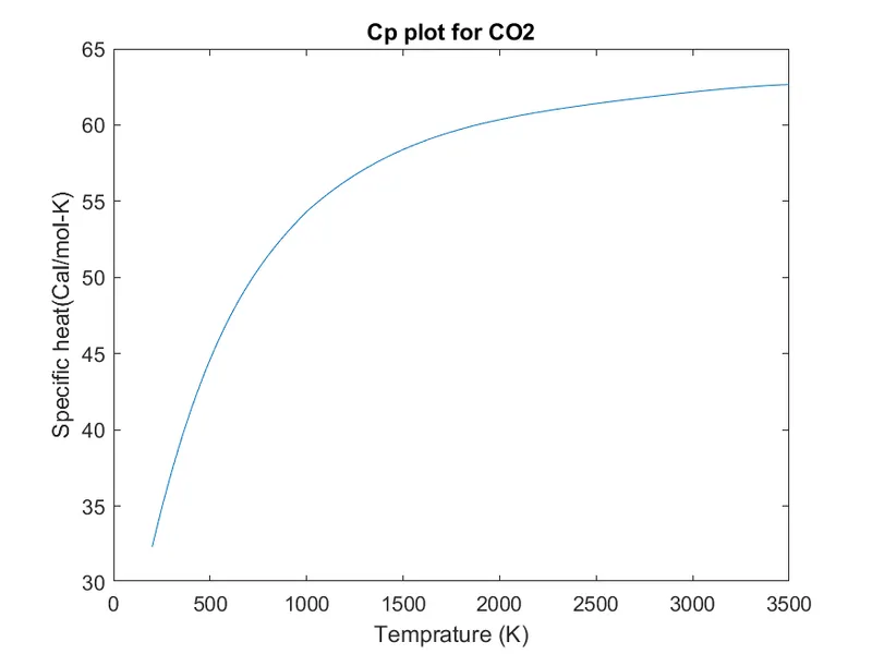
- Plot the Cp, Enthalpy and Entropy for the local temperature range (low temperature: high temperature) specific for each species.
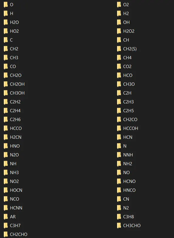
- Save the plots as images with appropriate names and dump them in separate folders for each species with suitable name. All these should be generated automatically.
THEORY:
Parsing in computer languages refers to syntactic analysis of the input code into its components parts in order to facilitate the writing of compilers and interpreters. It can be used to describe split or separation.
Parsing a file means reading in a data stream of some sort and building an in memory model of the semantic content of that data. This aims at facilitating perfoming some kind of transformation on the data.
NASA came up with polynomials that can be used to evaluate thermodynamic properties such as Cp, H and S. They have also documented the co-efficients that are required to evaluate these polynomials for 1000+ species. The Cp, H and S values can be calculated from the below formulaes.

PROGRAM:
The codes are done using MATLAB.
clc
clear all
close all
diary on %used to save all the contents of command window into a word file

%initialising universal gas constant
R = 8.314;

%opening the given file
f = fopen('THERMO.dat');
line = fgetl(f);
tline = fgetl(f); %extracting the global temprature range

A = strsplit(tline,' ');

%initialising the temprature values
Global_temp_low = str2double(A{2});
Global_temp_mid = str2double(A{3});
Global_temp_high = str2double(A{4});

%skipping the comment lines in the given file
for i =1:3
    line = fgetl(f);
end

%running the loop for 53 different species in the file
for data = 1:53
    line = fgetl(f);
    a = strsplit(line,' ');
    species_name(data) = a(1);
    F = strfind(line,'G');
    %storing the local temprature values
    tlow = str2double(line(F+4:55));
    thigh = str2double(line(F+13:65));
    tmid = str2double(line(F+23:75));

    %extracting the 14 co efficients and storing them in h.
    line = fgetl(f);
    F = strfind(line,'E');
    h(1) = str2double(line(1:F(1)+3));
    for i = 2:5
        h(i) = str2double(line(F(i-1)+4:F(i)+3));
    end

    line = fgetl(f);
    F = strfind(line,'E');
    h(6) = str2double(line(1:F(1)+3));
    for i = 7:10
        h(i) = str2double(line(F(i-6)+4:F(i-5)+3));
    end

    line = fgetl(f);
    F = strfind(line,'E');
    h(11) = str2double(line(1:F(1)+3));
    for i = 12:14
        h(i) = str2double(line(F(i-11)+4:F(i-10)+3));
    end

    T = linspace(tlow,thigh,500);
    %Cp, H & S values are calculated for every T and stored in an array
    for m = 1:length(T)
        if T(m) < tmid
            Cp(m) = (h(8)+h(9)*T(m)+h(10)*T(m)^2+h(11)*T(m)^3+h(12)*T(m)^4)*R;
            H(m) = (h(8)+(h(9)*T(m))/2+(h(10)*(T(m)^2))/3+(h(11)*(T(m)^2))/4+(h(12)*(T(m)^2))/5+(h(13)/T(m)))*T(m)*R;
            S(m) = (h(8)*log(T(m))+h(9)*T(m)+(h(10)*(T(m)^2))/2+(h(11)*(T(m)^2))/3+(h(12)*(T(m)^2))/4+h(14))*R;
        else
            Cp(m) = (h(1)+h(2)*T(m)+h(3)*T(m)^2+h(4)*T(m)^3+h(5)*T(m)^4)*R;
            H(m) = (h(1)+(h(2)*T(m))/2+(h(3)*(T(m)^2))/3+(h(4)*(T(m)^2))/4+(h(5)*(T(m)^2))/5+(h(6)/T(m)))*T(m)*R;
            S(m) = (h(1)*log(T(m))+h(2)*T(m)+(h(3)*(T(m)^2))/2+(h(4)*(T(m)^2))/3+(h(5)*(T(m)^2))/4+h(7))*R;
        end
    end
    %Creating a folder
    thermo_data = sprintf('%s',species_name{data});
    mkdir('NASA_thermodynamics_plots',thermo_data);

    %Cp plotting
    figure(1)
    plot(T,Cp)
    xlabel('Temprature (K)')
    ylabel('Specific heat(Cal/mol-K)')
    title(['Cp plot for ',species_name{data}])
    saveas(gcf,fullfile('NASA_thermodynamics_plots',thermo_data,'Specific_heat_curve.png'))

    %H plotting
    figure(2)
    plot(T,H)
    xlabel('Temprature (K)')
    ylabel('Enthalpy(KCal/mol)')
    title(['H plot for ',species_name{data}])
    saveas(gcf,fullfile('NASA_thermodynamics_plots',thermo_data,'Enthalpy_curve.png'))

    %S plotting
    figure(3)
    plot(T,S)
    xlabel('Temprature (K)')
    ylabel('Entropy(Cal/mol-K)')
    title(['S plot for ',species_name{data}])
    saveas(gcf,fullfile('NASA_thermodynamics_plots',thermo_data,'Entropy_curve.png'))

    %Molecular mass Calculation
    elements = {'H','C','N','O','A'};
    Atomic_Weight = [1.0079 12.0107 14.0067 15.999 39.948];
    w(data) = 0; %initialising to 0 for every species

    for q = 1:length(species_name{data})
        for p = 1:length(elements)
            if strcmp(species_name{data}(q),elements(p))==1 %compairing each charecter with the elemnt array
                w(data) = w(data) + Atomic_Weight(p);
                position = p;
            end
        end
            n = str2double(species_name{data}(q)); %check for numerical values of the same element
            if n>1
                w(data) = w(data) + Atomic_Weight(position)*(n-1);
            end
    end
    %printing values in the command window
    sprintf('Molecular Weight of %s : %fu',species_name{data},w(data))

end

diary off
fclose(f);
EXPLANATION OF THE CODE:
In the above code,
- Initially the file is opened using fopen.
- The global temprature range are extracted using fgetl and strsplit is used to split the line. Then each temprature is initialised to a variable.
- Then a loop is run for 53 different species present in the given data file.
- After the local temrature values are assigned, the 14 coefficients are extracted and stored in h.
- The values of Cp, H & S are xalculated using the given formulaes and their plots are plotted w.r.to T .
- Then the molecular weights are calculated by character comparision using strcmp and the weights are added up.
- The molecular weights of each species are displayed in the command window using sprintf and the screenshot if the displayed values are attached in the OUTPUT section.
- Finally the file was closed using fclose.
OUTPUT:
The screenshot of the folder containing all the graphs is given below:
Plots of O2:
Plots of N2:
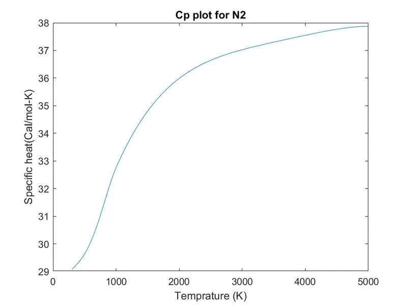
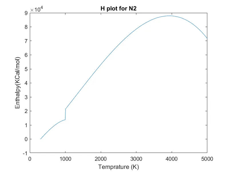
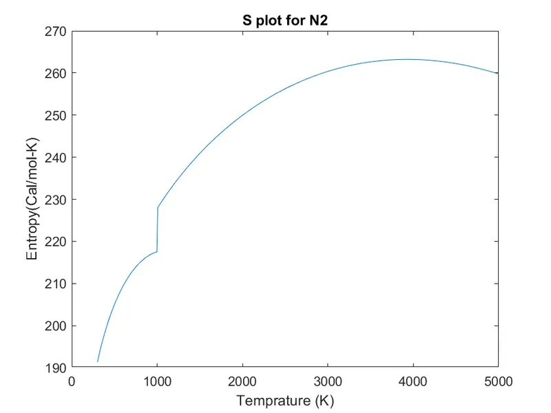
Plots of CO2:
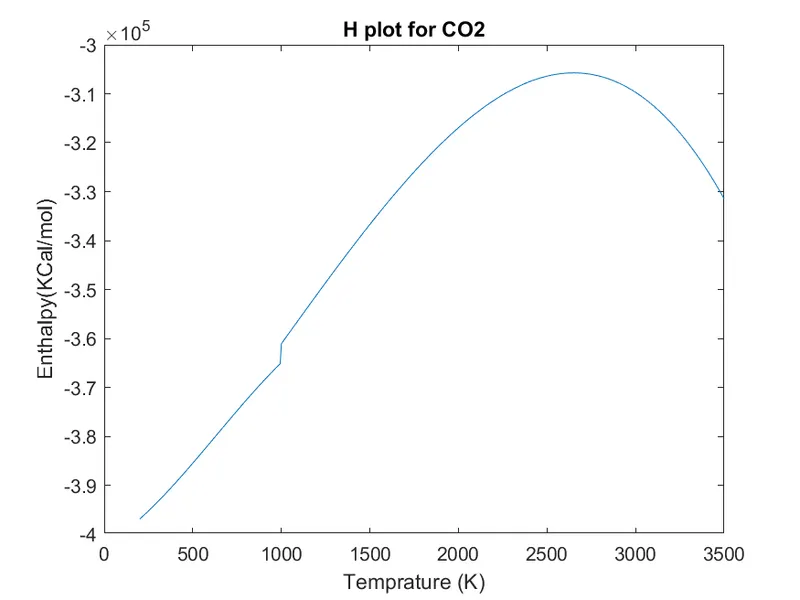
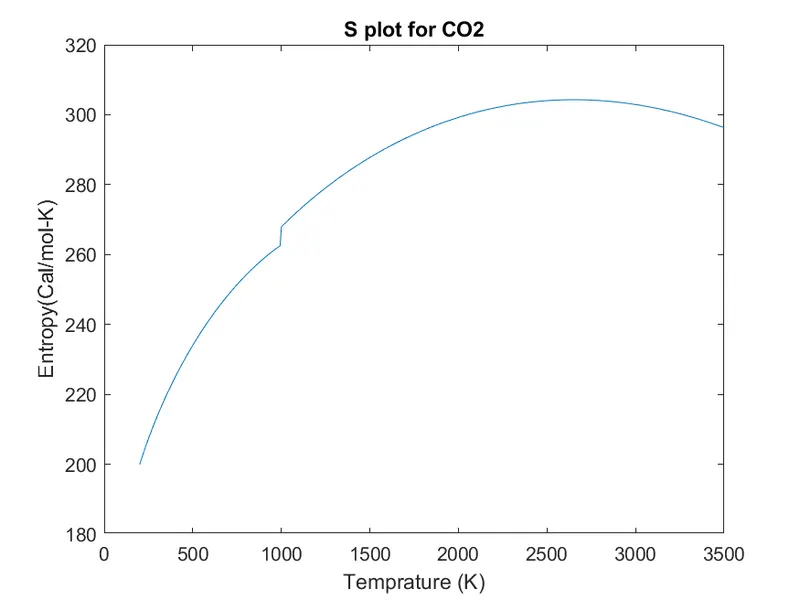
The MATLAB command window contents are:
CONCLUSION:
The above experiment was completed successfully. The simulation was done and all the required outputs are attached above.