Week 4.1 - Genetic Algorithm
AIM - To write down the code to optimize the stalagmite function and to find the global maxima and minima/local maxima and minima
EXPLAINATION-
- GENETIC ALGORITHM- Genetic algorithm is a method to solve the optimization problem by natural selection through the process of biological evolution. It modifies repeatedly on the population of individual solutions. At each steps genetic algorithm select the current population randomly to predict next generation population producing i.e. parents and uses them to produce the children for the next generation.
- STOPPING CRITERIA GA- GA stop when it reaches the maximum number of generation, such as when the generation reaches to the predefine value, it stop and provide the best solution in the last generation or if the best solution during the evolution process does not change to the better value for the predefine value of the generation.
- SYNTAX FOR ga- ‘ga’ is genetic algorithm function which is preload in matlab software, it can be encoded in the program instead for writing full sentence, it look discreet in the line commands and not much hassle to write in the programs, matlab can recognize this command.
- SIGNIFICANCE OF RUNNING MULTIPLE ITERATIONS
PROGRAM
FILE- ga_main.m
clear all
close all
clc
% Defining our search space
x = linspace(0,0.6,150);
y = linspace(0,0.6,150);
% creating a 2Dimensional mesh
[xx, yy] = meshgrid(x, y);
% Evaluation the stalagmite function
for i = 1:length(xx)
for j = 1:length(yy)
input_vector(1) = xx(i,j);
input_vector(2) = yy(i,j);
f(i,j) = stalagmite(input_vector);
end
end
surfc(xx,yy,f)
shading interp
[inputs, fval] = ga(@stalagmite,2)
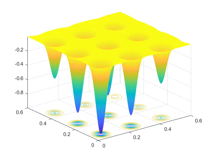
- Clear all ,close all and clc is written first before starting the program because if any numerical values, variables etc, are present then the final result may get error or it may get manipulated. It will close it out.
- % Defining our search space
x = linspace(0,0.6,150);
y = linspace(0,0.6,150);
It is the input data of x and y in one-dimension, so we have to change it through two-dimension through meshgrid which shown below.
% creating a 2Dimensional mesh
[xx, yy] = meshgrid(x, y);
- % Evalution the stalagmite function
for i = 1:length(xx)
for j = 1:length(yy)
input_vector(1) =xx(i,j);
input_vector(2) =yy(i,j);
f(i,j) = stalagmite(input_vector);
end
end
- for i = 1:length(xx)
‘i’ is the variable of(xx)
1:length(xx) means it given the value of 0 to 150 at an equal interval of 0.6 value every time.
- for j = 1:length(yy)
‘j’ is the variable of(yy)
1:length(yy) means it given the value of 0 to 150 at an equal interval of 0.6 value every time.
- input_vector(1) =xx(i,j);
input_ vector(1) is a row vector which contains 2 columns of ‘x’ and put them in array(i,j)
- input_vector(2) =yy(i,j);
input_ vector(2) is a row vector which contains 2 columns of ‘y’ and put them in array(i,j)
- f(i,j) = stalagmite(input_vector);
stalagmite is function which takes the input_vector and calculate ‘F’
as it is shown below.
This function code is coded in the new script with the same function name and the file name.
FILE- stalagmite.m
function [F] = stalagmite(input_vector)
% Defining input conditions
x = input_vector(1);
y = input_vector(2);
% Solving the equations to obtain the values of the function
f1x = (sin((5.1*pi*x)+0.5))^6;
f1y = (sin((5.1*pi*y)+0.5))^6;
f2x = exp(-4*log(2)*(((x-0.0667)^2)/0.64));
f2y = exp(-4*log(2)*(((y-0.0667)^2)/0.64));
F = -(f1x*f1y*f2x*f2y);
End
- function [F] = stalagmite(input_vector)
f(i,j) = stalagmite(input_vector);
which is coded in ga-main.m file
- % Defining input conditions
x = input_vector(1);
y = input_vector(2);
input_vector(1) =xx(i,j);
input_vector(2) =yy(i,j);
which is coded in ga-main.m file
- % Solving the equations to obtain the values of the function
f1x = (sin((5.1*pi*x)+0.5))^6;
f1y = (sin((5.1*pi*y)+0.5))^6;
f2x = exp(-4*log(2)*(((x-0.0667)^2)/0.64));
f2y = exp(-4*log(2)*(((y-0.0667)^2)/0.64));
F = -(f1x*f1y*f2x*f2y);
End
This the given formula to calculate the equation of the variable f1x,f1y,f2x and f2y.
The fitness function will find the value of ‘f’ by varying the value of input arguments x and y and find the value of f as minimum as possible. It’s compare’s the fitness value with optimize value of ‘f’ for every iteration to find the good fit.
After stalagmite function,to optimize the final program a new function is defined ‘get_stalagmite’ which contains ‘for loop’ and ‘meshgrid commands’.
This function code is coded in the new script with the same function name and the file name.
FILE- get_stalagmite
function [f] = get_stalagmite(x,y)
[xx,yy] = meshgrid(x,y);
for i = 1:length(xx)
for j = 1:length(yy)
input(1) = xx(i,j);
input(2) = yy(i,j);
f(i,j) = stalagmite(input);
end
end
FILE- ga_statistics (Final Program)
clear all
close all
clc
x = linspace(0,0.6,150);
y = linspace(0,0.6,150);
num_cases = 50
f = get_stalagmite(x,y);
tic
% Study1 - Satistical behavior
for i = 1:num_cases
[inputs, fopt(i)] = ga(@stalagmite, 2);
xopt(i) = inputs(1);
yopt(i) = inputs(2);
end
study1_time = toc;
figure(1)
subplot(2,1,1)
hold on
surfc(x, y, f)
shading interp
plot3(xopt,yopt,fopt,'marker','o','markersize',5,'MarkerFaceColor','r')
title('Unbounded inputs')
subplot(2,1,2)
plot(fopt)
xlabel('iterations')
ylabel('Function minimum')
tic
% Study2 - Statistical behavior- with upper and lower bounds
for i = 1:num_cases
[inputs,fopt(i)] = ga(@stalagmite,2,[],[],[],[],[0;0],[1;1]);
xopt(i) = inputs(1);
yopt(i) = inputs(2);
end
study2_time = toc;
figure(2)
subplot(2,1,1)
hold on
surfc(x, y, f)
shading interp
plot3(xopt,yopt,fopt,'marker','o','markersize',5,'markerfacecolor','r')
title('Bounded inputs')
subplot(2,1,2)
plot(fopt)
xlabel('Iterations')
ylabel('Function minimum')
% Study3 increasing GA iterations
options = optimoptions('ga')
options = optimoptions(options,'populationsize',300)
tic
for i = 1:num_cases
[inputs,fopt(i)] = ga(@stalagmite,2,[],[],[],[],[0;0],[1;1],[],[],options);
xopt(i) = inputs(1);
yopt(i) = inputs(2);
end
study3_time = toc;
figure(3)
subplot(2,1,1)
hold on
surfc(x, y, f)
shading interp
plot3(xopt,yopt,fopt,'marker','o','markersize',5,'markerfacecolor','r')
title('Bounded inputs with Increased populationsize')
subplot(2,1,2)
plot(fopt)
xlabel('Iterations')
ylabel('Function minimum')
EXPLAINATION-
- Clear all ,close all and clc is written first before starting the program because if any numerical values, variables etc, are present then the final result may get error or it may get manipulated. It will close it out.
- x = linspace(0,0.6,150);
y = linspace(0,0.6,150);
num_cases = 50
f = get_stalagmite(x,y);
x = linspace(0,0.6,150);
y = linspace(0,0.6,150);
Two linspace command is used to find out the values of both x and y in search space.
num_cases = 50
It will run the genetic algorithm 50 times.
f = get_stalagmite(x,y);
get_stalagmite(x,y) function generate stalagmite function.
tic
- % Study1 - Statistical behavior
for i = 1:num_cases
[inputs, fopt(i)] = ga(@stalagmite, 2);
xopt(i) = inputs(1);
yopt(i) = inputs(2);
end
study1_time = toc;
figure(1)
subplot(2,1,1)
hold on
surfc(x, y, f)
shading interp
plot3(xopt,yopt,fopt,'marker','o','markersize',5,'MarkerFaceColor','r')
title('Unbounded inputs')
subplot(2,1,2)
plot(fopt)
xlabel('iterations')
ylabel('Function minimum')
- tic- The function record the current time.
Study1 – Statistical behavior
for i = 1:num_cases
‘for loop’ is the repetition control from 1 to number of cases of a given input i.e 1 to 50 times.
- study1_time = toc;
The function uses the recorded value of the to calculate the elapsed time.
[inputs, fopt(i)] = ga(@stalagmite, 2);
xopt(i) = inputs(1);
yopt(i) = inputs(2);
In this part ‘ga’ command is used and the stalagmite function with 2 inputs.
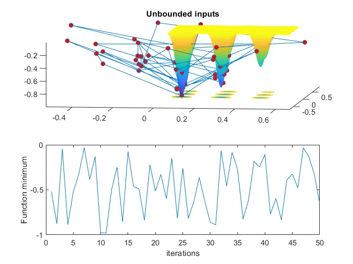
Study1 plotting graphical representation.
- Subplot-The subplot command is used to create the multiple plots in the same figure or graphs.
- hold on- It adds 2nd line plot without deleting the existing line plot.
- surfc(x, y, f)
This command generate the 3-D graphics of the surface of 360 degree view to analyze the surface structure of x,y and fitness function value (f).
- shading interp- It varies color in each line segment and face by interpolating the colormap.
- plot3(xopt,yopt,fopt,'marker','o','markersize',5,'markerFaceColor','r')
plot3 command is for x,y and optimum value of ga prediction over 50 studies.
- title('Unbounded inputs')- Title command is a text which can be named,values and modifies the appearance i.e unbounded inputs.
- subplot(2,1,2)
The 2nd subplot is plotted as a function of iterations.
- plot(fopt)- This is the plot for fitness optimize value.
- xlabel('iterations')
ylabel('Function minimum')
X-LABEL- This command which label x-axis in the graphical representation
Y-LABEL- This command which label y-axis in the graphical representation.
study1_time = 5.3921
tic
- % Study2 - Statistical behavior- with upper and lower bounds
for i = 1:num_cases
[inputs,fopt(i)] = ga(@stalagmite,2,[],[],[],[],[0;0],[1;1]);
xopt(i) = inputs(1);
yopt(i) = inputs(2);
end
study2_time = toc;
figure(2)
subplot(2,1,1)
hold on
surfc(x, y, f)
shading interp
plot3(xopt,yopt,fopt,'marker','o','markersize',5,'markerfacecolor','r')
title('Bounded inputs')
subplot(2,1,2)
plot(fopt)
xlabel('Iterations')
ylabel('Function minimum')
- tic- The function record the current time.
- for i = 1:num_cases
‘for loop’ is the repetition control from 1 to number of cases of a given input i.e 1 to 50 times.
- [inputs,fopt(i)] = ga(@stalagmite,2,[],[],[],[],[0;0],[1;1]);
xopt(i) = inputs(1);
yopt(i) = inputs(2);
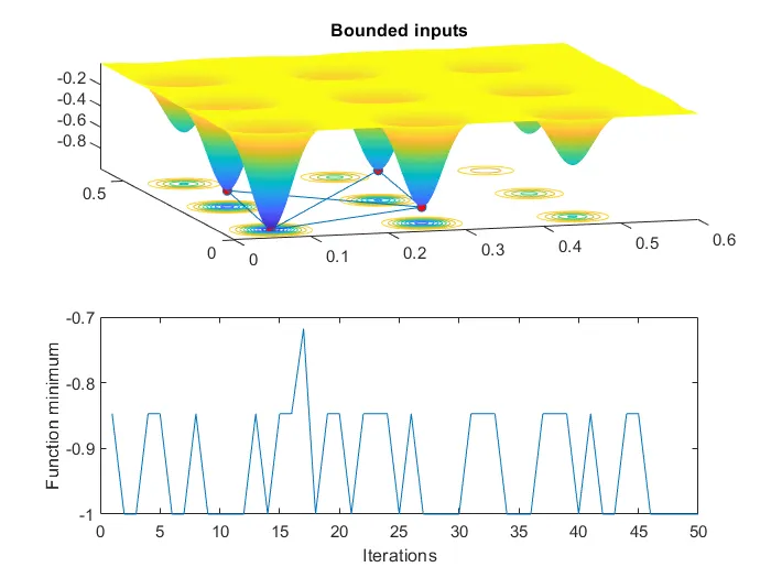
In this part ‘ga’ command is used and the stalagmite function with 2 inputs with lower bound and upper bound i.e upper limit boundary and lower lower limit boundary which gives the fitness value with that range in the plot.
- study2_time = toc;
The function uses the recorded value of the to calculate the elapsed time.
- Subplot-The subplot command is used to create the multiple plots in the same figure or graphs.
- hold on- It adds 2nd line plot without deleting the existing line plot.
- surfc(x, y, f)
This command generate the 3-D graphics of the surface of 360 degree view to analyze the surface structure of x,y and fitness function value (f).
- shading interp- It varies color in each line segment and face by interpolating the colormap.
- plot3(xopt,yopt,fopt,'marker','o','markersize',5,'markerFaceColor','r')
plot3 command is for x,y and optimum value of ga prediction over 50 studies.
- title('Bounded inputs')- Title command is a text which can be named, values and modifies the appearance i.e bounded inputs.
- subplot(2,1,2)
The 2nd subplot is plotted as a function of iterations.
- plot(fopt)- This is the plot for fitness optimize value.
- xlabel('iterations')
ylabel('Function minimum')
X-LABEL- This command which label x-axis in the graphical representation
Y-LABEL- This command which label y-axis in the graphical representation.
- study2_time = 66.4999
% Study3 increasing GA iterations
options = optimoptions('ga')
options = optimoptions(options,'populationsize',300)
tic
for i = 1:num_cases
[inputs,fopt(i)] = ga(@stalagmite,2,[],[],[],[],[0;0],[1;1],[],[],options);
xopt(i) = inputs(1);
yopt(i) = inputs(2);
end
study3_time = toc;
figure(3)
subplot(2,1,1)
hold on
surfc(x, y, f)
shading interp
plot3(xopt,yopt,fopt,'marker','o','markersize',5,'markerfacecolor','r')
title('Bounded inputs with Increased populationsize')
subplot(2,1,2)
plot(fopt)
xlabel('Iterations')
ylabel('Function minimum')
- options = optimoptions('ga')
options = optimoptions(options,'populationsize',300)
optimoptions- This command is to organize option by solver.
- options = optimoptions('ga')
This through (‘ga’) command.
- options = optimoptions(options,'populationsize',300)
This through (‘populationsize’300) command.
[NOTE - The rest command line is same in study1 and study2,which I have explained.]
The populationsize will be increased because the initial size is too small then it wouldn’t find out the global maxima or minima.
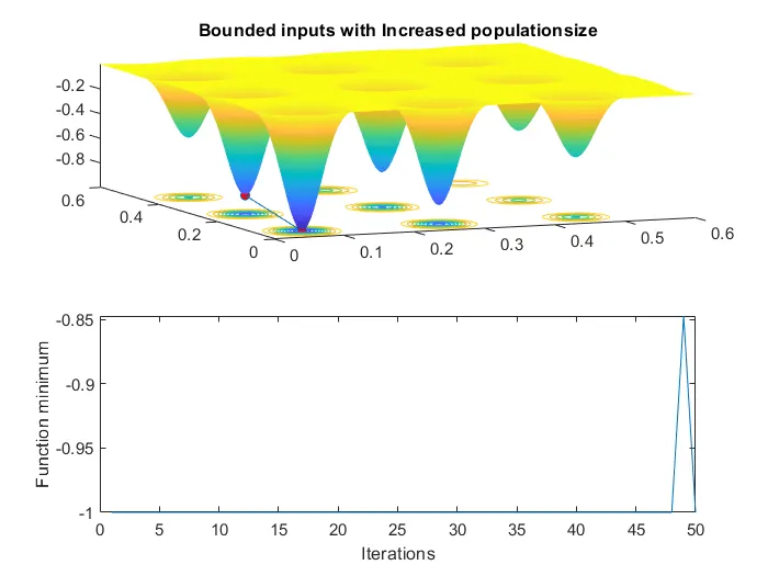
- study3_time = 26.4899