Week 3 - Solving second order ODEs
AIM – To solve ODE and calculate numerical values through programming by generating animation of simple pendulum and plotting the graphical representation through MATLAB.
PROGRAMMING CODE
File name – ode_func.m
% A function program of ODE
function [dtheta_dt] = ode_func(t,theta,b,g,l,m)
theta1 = theta(1)
theta2 = theta(2)
dtheta1_dt = theta2;
dtheta2_dt = -(b/m)*theta2 - (g/l)*sin(theta1);
dtheta_dt =[dtheta1_dt; dtheta2_dt];
end
EXPLAINATION –
The file function name and the file name is saved should be same.
- ode_func
- dtheta1_dt = theta2;
consider -
theta = theta1
ANS - dtheta_dt = dtheta1_dt = theta2
- dtheta2_dt = -(b/m)*theta2 - (g/l)*sin(theta1);
Given –
d^2_theta_dtheta^2 + b/m*(dtheta_dt) + (g/l)*sin(theta) = 0
Solving -
d^2_theta1_dt + b/m*(dtheta1_dt) + (g/l)*sin(theta1) = 0
dtheta2_dt + (b/m)*theta2 + (g/l)*sin(theta1) = 0
ANS - dtheta2_dt = -(b/m)*theta2 – (g/l)*sin(theta1)
- dtheta_dt =[dtheta1_dt; dtheta2_dt]
d/dt[theta1;theta2] = [theta2; -(b/m)*theta2 –(g/l)*sin(theta)]
ANS - dtheta_dt = [dtheta1_dt; dtheta2_dt]
File name – ode_main.m
% solving second order
clear all
close all
clc
b = 0.02;
g = 9.81;
l = 1;
m = 0.1;
% intial condition
theta_0 = [0;5];
% time points
t_span = linspace(0,10,100);
% solve ODE
[t, result] = ode45(@(t,theta)ode_func(t, theta, b,g,l,m),t_span, theta_0);
% Plotting
plot(t,result(:,1))
hold on
plot(t,result(:,2))
ylabel('plot')
xlabel('time')
% For loop
ct = 1
for i=1:length(t)
x=l*sin(result(i,1));
y=-l*cos(result(i,1));
% Plotting the animation
figure(2)
plot([-1,1],[0,0])
plot([0,x],[0,y])
hold on
plot(x,y,'o','markersize',20,'markerfacecolor','r')
axis([-1.5 1.5 -1.5 1.5])
pause(0.03)
M(ct) = getframe(gcf);
ct = ct+1;
hold off
end
% Animation of the pendulum
movie(M)
videofile = VideoWriter('ode_main.avi','Uncompressed AVI');
open(videofile)
writeVideo(videofile,M)
close(videofile)
EXPLAINATION –
- Clear all ,close all and clc is written first before starting the program because if any numerical values, variables etc, are present then the final result may get error or it may get manipulated.It will close it out.
- b = 0.02;
g = 9.81;
l = 1;
m = 0.1;
where as:-
b = damping coefficient
g = gravity (m/s^2)
l = length of the spring (m)
m = mass of the bob (kg)
- % intial condition
theta_0 = [0;5];
where as:-
angular displacement is 0
angular velocity is 5
It is represented in column matrix
- % time points
t_span = linspace(0,10,100);
t_span is time of initial time of the pendulum oscillation to final time of the oscillation from 0 to 10 seconds of 100 times of iteration.
For clear picture you can go to workspace window and double click on the t-span it will show you the iteration with time values.
- % solve ODE
[t, result] = ode45(@(t,theta)ode_func(t, theta, b,g,l,m),t_span, theta_0);
ode45 - Ode45 is inbuilt differential solver,it is a function in Matlab to solve ordinary or partial differential equations.The function of ode45 takes 3 inputs which is to be integrated.
t_span and the initial conditions.[t,result].
- % Plotting
plot(t,result(:,1))
hold on
plot(t,result(:,2))
ylabel('plot')
xlabel('time')
- plot(t,result(:,1))
[t, result] = ode45(@(t,theta)ode_func(t, theta, b,g,l,m),t_span, theta_0);
(:,1) means it first order derivative.
- plot(t,result(:,2))
[t, result] = ode45(@(t,theta)ode_func(t, theta, b,g,l,m),t_span, theta_0);
(:,2) means it is second order derivative.
- ylabel('plot')
xlabel('time')
In graphical representation x-axis is given as(time) and y-axis is given as(plot).
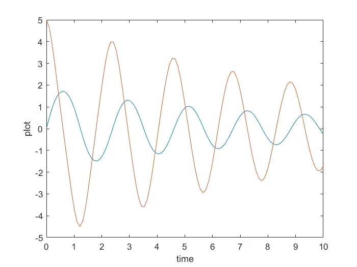
Red curve line showing above the graph is angular velocity.
Blue curve line showing above the graph is angular displacement.
% For loop
ct = 1
for i=1:length(t)
x=l*sin(result(i,1));
y=-l*cos(result(i,1));
FOR LOOP- ‘for loop’ is the command which is used to assign a range from the initial step to final step with the increment. It is used as a counter with in a program to count the number of calculations.
ct is counter loop which is added before the ‘for loop’ code program starts.
x=l*sin(result(i,1));
y=-l*cos(result(i,1));
this are the coordinates of x-axis and y-axis of a pendulum in the program prompt.
% Plotting the animation
figure(2)
plot([-1,1],[0,0])
plot([0,x],[0,y])
hold on
plot(x,y,'o','markersize',20,'markerfacecolor','r')
axis([-1.5 1.5 -1.5 1.5])
pause(0.03)
M(ct) = getframe(gcf);
ct = ct+1;
hold off
end
plot([0,x],[0,y])
(0) is the origin in x direction and (0) is the origin in y direction respectively.
plot(x,y,'o','markersize',20,'markerfacecolor','r')
x and y is the coordinates.
‘O’ is the bob of the pendulum.
‘markersize’ is the size of the bob,given input is 20.
‘markerfacecolor,’,‘r’ is the color of the bob and r represent red color.
pause(0.03) - Pause command is used to stop the command for the certain time.
ct = ct+1
add + 1 to the final step to ct variable,this will increment the frame every time for loop to run.
% Animation of the pendulum
movie(M)
videofile = VideoWriter('ode_main.avi','Uncompressed AVI');
open(videofile)
writeVideo(videofile,M)
close(videofile)
- movie(M)- To create a movie this input is given at the beginning of the program.
- videofile = VideoWriter('ode_main.avi','Uncompressed AVI');
videoWrite command is to give the format of the video with videofile name .avi
- open(videofile)- This command is used to open the file in the media player.
- writeVideo(videofile,M)- This command is to write video frames.
- close(videofile)- This command is used to close the video in the media player.
https://drive.google.com/file/d/1teQJJlr2c1rgk2BXFfideuWsTrXJzM2N/view?usp=sharing