Week 4.1 - Genetic Algorithm

Aim

Write a code in MATLAB to optimise the stalagmite function and find the global maxima of the function.

Objectives

• Clearly expalin the concept of genetic algorithm and also explain the syntax for ga in MATLAB.
• Make sure that the code gives the same output, even if it is made to run several times.
• Plot graphs for all 3 studies and for F maximum vs no. of iterations. Title and axes labels are a must, legends could be shown if necessary.

Methodology

Theory

Global optimization program is a program that modify all design parameters and rearrange the combinations to give maximum effectiveness. It deals with how to minimize and maximize perticular function which depends on multiple input parameters. The objectives of optimization study is to determine the global maxima/minima by using the genetic algorithm. Here we use the stalagmite function which we wanted to optimise and find out global maxima. A stalagmite function is a function with which we are generating the values over a stalagmite kind of surface to find out the local and global maxima and minima of that particular given function. Matlab provide inbuilt genetic algorithm function to find out the local and global maxima and minima.

Genetic Algorithm (GA)

Genetic algorithm is a search method which is inspired from the Darvin's Theory of Evolution. This resembles the theory of natural selection , which describe the survival of the fittest that means the fittest individual is selected for the reproduction inorder to produce offsprings for the next generation.
Theory of natural selection involves the selection of fittest individuals from a population and production of offsprings using the individuals and inherit the characteristics of them to next generation. If parents have better fitness, their offspring will be better than parents and have a better chance at surviving. Keeps on iterating this selection process we get a generation with fittest individual at the end.

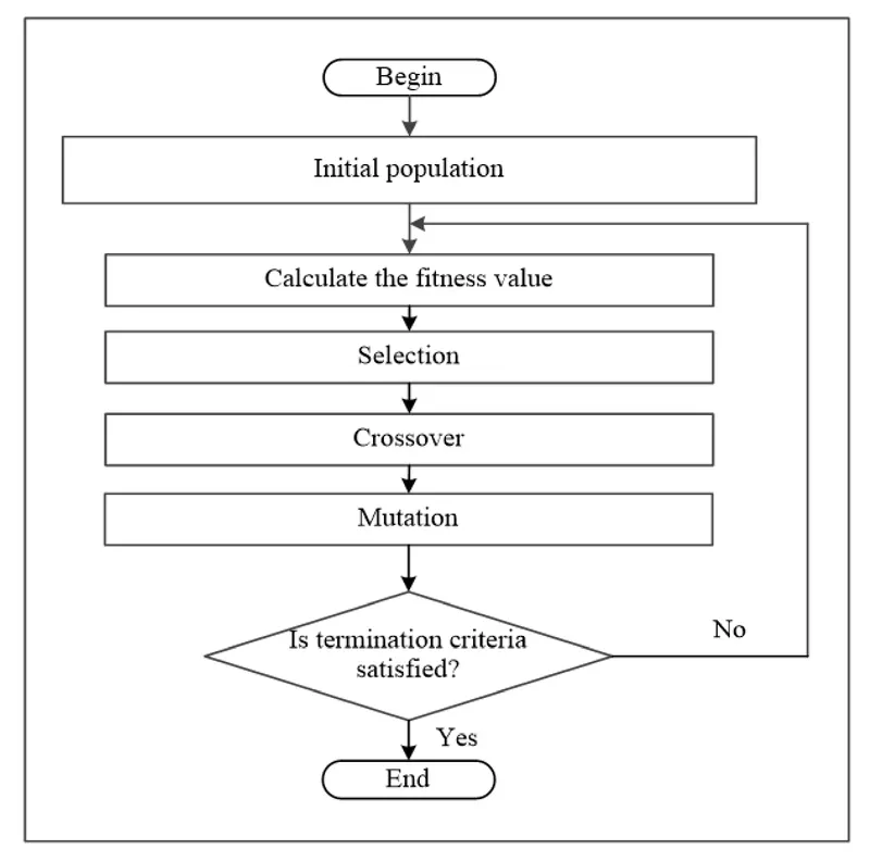
Genetic algorithm involves 5 phases

1. Initial Population
2. Fitness function
3. Selection
4. Crossover
5. Mutation

Flowchart Showing the GA Phases

1. Initial Population

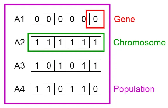
It is the population on which Genetic algorithm (GA) carried out. It is considered as a set of individual and each individual is a solution to the problem we wanted to solve. Each of this individual consist of a set of parameters (represent variables x,y here) called genes. Genes joined to form a string called Chromosom(here represent Solution). In GA genes are represented using the binary values(string of 1s and 0s) and the encoded string called a chromosom.

2. Fitness Function

It is the function that determines how fit an individual is, that is the ability of the individual to survive and compete with others. It provide a fitness score to each individual and based on this an individual will be selected for reproduction.

3. Selection

In this phase select the fittest individual and allow them to transfer its genes to next generation. Based onthe fitness score Pairs of individuals selected and allow them to reproduce. individuals with high fitness score have more chance to be selected for reproduction.

4. Crossover

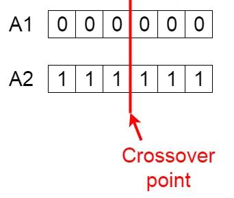
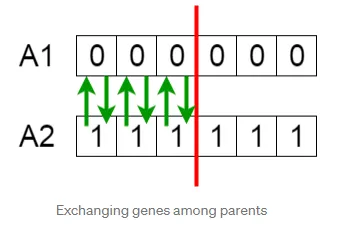
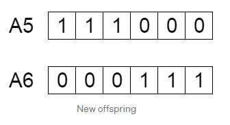
It is the most importent phase in GA as it choose a crossover point at random within the genes of each pair of parents to be mated. Let the crossover point be at 3 and the new generation is created by exchangeing genes until the crossover point reached. Crossover takesplace as shown below.

5. Mutation

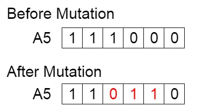
Here new offsprings are created by inserting genes randomly. The probability of happening this is very low. But the mutation helps to maintain diversity within the population and prevent premature convergence.

Termination of GA

The termination of algorithm happens when the population is converged, that is the population does not produce offspring which are significantly different from the previous generation. Then it is said that GA has provided a set of solutions to the problem.

Termination command detrermine when to stop the GA solver. The stopping conditions are selected by using the command "opts=optmoptions("ga","options")"

options includes

• MaxGenerations - The algorithm stops when the no.of generations reaches MaxGenerations.
• MaxTime - The algorithm stops after running for an amount of time in seconds equal to MaxTime.
• FitnessLimit - The algorithm stops when the value of fitness function for the best point in the current population is less than or equal to FitnessLimit.
• MaxStallGenerations - The algorithm stops when the average relative change in the fitness function value over MaxStallGenerations is less than Function tolerance
• MaxStallTime - The algorithm stops when there is no improvement in the objective function during an interval of time in seconds equal to MaxStallTime.
• FunctionTolerance - The algorithm runs until the average relative change in the fitness function value over MaxStallGenerations is less than function tolerance.
• ConstraintTolerance - It is not used as stopping criterion. It used to determine the feasibility with respect to nonlinear constraints.

Genetic Algorithm Syntax

1. x = ga(fun,nvars) It helps to find local unconstraints minimum,"x", to the function, "fun". "nvars" represent no.of design variables of function, "fun".

2. x=ga(fun,nvars,A,b,Aeq,beq,lb,ub) Here solution is found between an upper and lower bounds(ub,lb). ie `lb<=x<=ub`. here local minima,"x", of the function "fun" found out between the constraints, Linear inequality `A*x<=b`, Linear equalities `Aeq*x=beq` , `lb<=x<=ub` (upper and lower limits). If linear inequality and linear equality are not exist then use [ ] in their respective positions(x=ga(fun,nvars,[ ],[ ],[ ],[ ],lb,ub))

• fun - function
• nvars - no. of design variables of function.
• A- linear inequality constraints
• b- linear inequality constraints
• Aeq - linear equality constraints
• beq - linear equality constraints
• lb - lower limit
• ub- upper limit

3. x=ga(fun,nvars,A,b,Aeq,beq,lb,ub,nonlcon,intcon,options) Here the default optimization parameters replaced by the value in the "options". here inadition to the constaraints explained above there is a nonlinear constraints "nonlcon". And also "intcon" which takes integer values.

• nonlcon - non linear constraints
• intcon - The variable listed in intcon takes integer values.
• options - default optimization options replaced by value in the option created by using the code "optimoptions"

if no constraints exist use [ ] in their respective positions.

The GA function runs multiple iterations inorder to provide the better and smooth result. significance of running multiple iterations is it helps in determining the authenticity of the results we get. Running the function multiple times and geting the same results every time indicate the value obtained is true and authentic.

Equations Used

Stalagmite function

`f(x,y)=-(f_(1x)*f_(2x)*f_(1y)*f_(2y))`

-ve sign given is to find out the maximum value of function

`f_(1x)=(sin(5.1pix+0.5))^6`

`f_(1y)=(sin(5.1piy+0.5))^6`

`f_(2x)=exp[-4ln(2)((x-0.0667)^2)/0.64]`

`f_(2y)=exp[-4ln(2)((y-0.0667)^2)/0.64]`

MATLAB CODE

Function Code

% Stalagmite function creation
% ga normally finds the minimum value of a function, so inorder to find the
% maximum value use a -ve sign in the stalagmite function equation

function [stalagmite]= stalagmite(A)
        f1_x=(sin(5.1*pi*A(1)+0.5))^6;
        f1_y=(sin(5.1*pi*A(2)+0.5))^6;
        f2_x=exp(-4*log(2)*((A(1)-0.0667)^2)/0.64);
        f2_y=exp(-4*log(2)*((A(2)-0.0667)^2)/0.64);
        [stalagmite]=f1_x*f2_x*f1_y*f2_y*(-1);
end

Main Code

% Write a code in MATLAB to optimise the stalagmite function and find the global maxima of the function

clear all
close all
clc

% Defining the inputs which we wanted to be the search space
x=linspace(1,0.06,150);
y=linspace(1,0.06,150);

% creating a 2D array
[s, r]=meshgrid(x,y);

% Creating the stalagmite function values 
for i=1:length(x)
    for j=1:length(y)
        A(1)=s(i,j);
        A(2)=r(i,j);
        D(i,j)=stalagmite(A);
    end
end

% setting no. of iterations
n=50;
% Study-1 using the unbounded inputs
tic % for calculating time for run
% calling genetic algoritham(ga) to evaluate the stalagmite function and find
% the global maxima.(ga normally finds the minimum value of a function, so
% use a -ve sign in the stalagmite function at the time of creation of the function program in order to find maximum value)
% finding optimum values of the function and its coordinates and stored it
% in foptm and inputs (with out boundary conditions)
for i=1:n
    [inputs, foptm(i)]= ga(@stalagmite,2);
    x_optm(i)=inputs(1);
    y_optm(i)=inputs(2);
end

Time_for_study_1=toc

% plotting the values
figure(1)
subplot(2,1,1) % plotting multiple figures in a single plot
surf(x,y,D)
hold on
shading interp % for hiding the grid lines

% Showing the optimum/maximum value of function which obtained from running
% genetic algorithm
plot3(x_optm,y_optm,foptm,'marker','o','markersize',6,'MarkerFaceColor','r')
legend('function','foptum')
title('Study-1- Unbounded Inputs','Color','k')
xlabel('X-values','Color','b')
ylabel('Y-Values','Color','r')
hold off
subplot(2,1,2)
plot(foptm)
xlabel('Iterations')
ylabel('Maximum Value of function')


% Study-2 Bounded inputs by setting the Upper and lower bounds
% finding optimum values of the function and its coordinates and stored it
% in foptm and inputs (with boundary conditions)

tic

for i=1:n
    [inputs, foptm(i)]= ga(@stalagmite,2,[],[],[],[],[0;0],[1;1]);
    x_optm(i)=inputs(1);
    y_optm(i)=inputs(2);
end

Time_for_study_2=toc

figure(2)
subplot(2,1,1)
surf(x,y,D)
hold on
shading interp
plot3(x_optm,y_optm,foptm,'marker','o','markersize',6,'MarkerFaceColor','r')
legend('function','foptum')
title('Study-2-bounded Inputs','Color','k')
xlabel('X-values','Color','b')
ylabel('Y-Values','Color','r')
subplot(2,1,2)
plot(foptm)
xlabel('Iterations')
ylabel('Maximum Value of function')

% Study-3 bounded inputs(upper and lower limits) with incresed population
% size
% Setting the population size
option=optimoptions("ga");
option=optimoptions(option,'PopulationSize',300);

tic

% finding optimum values of the function and its coordinates and stored it
% in foptm and inputs (with boundary conditions and modified population size)
for i=1:n
    [inputs, foptm(i)]=ga(@stalagmite,2,[],[],[],[],[0;0],[1;1],[],[],option);
    x_optm(i)=inputs(1);
    y_optm(i)=inputs(2);
end

Time_for_study_3=toc

figure(3)
subplot(2,1,1)
surf(x,y,D)
shading interp
hold on
plot3(x_optm,y_optm,foptm,'marker','o','MarkerSize',6,'MarkerFaceColor','r')
legend('function','foptum')
title('Study-3 Bounded Input with Increased population size','Color','k')
xlabel('X-Value','Color','b')
ylabel('Y-Value','Color','r')
subplot(2,1,2)
plot(foptm)
xlabel('Itrations')
ylabel('Maximum Value of function')

Output And Code Explanation

• Created a input parameters which we wanted to be the search space x,y using the linspace command and using this x & y made a 2D array using meshgrid command.
• x=linspace(1,0.06,150);
• y=linspace(1,0.06,150);
• [s, r]=meshgrid(x,y);
• Using the values in 2D arrays [s, r], Created the stalagmite function values by putting the values of x and y variables in the stalagmite function equation. For this a column array [A] (1 row 2 colum metrix) is created and assign the value A(1) as x and A(2) as y. This is done by using a double for loop command.
• for i=1:length(x)
  for j=1:length(y)
  A(1)=s(i,j);
  A(2)=r(i,j);
  D(i,j)=stalagmite(A);
  end
  end

Study-1 using the unbounded inputs

• Set the no.of iterations n=50 for running the for loop 50 iterations.
• Called genetic algoritham(GA) in a for loop to evaluate the stalagmite function and tried to find out the global maxima.(ga normally finds the minimum value of a function, so use a -ve sign in the stalagmite function at the time of creation of the function program in order to find maximum value).
• [inputs, foptm(i)]= ga(@stalagmite,2) syntax of GA stalagmite is the function and 2 is the no. of variables of the function.
• Find out the optimum values of the function and its corresponding coordinates and stored it in foptm and inputs (with out boundary conditions) respectively. Inputs is a column vector(1 row and 2 column)
• foptm is the optimum value and x_optm and y_optm are their corresponding coordinates which assigned as follows x_optm=inputs(1), y_optm=inputs(2).
• Set a timer for calculating time for running the study 1 using tic toc command.
• Plot the 3D surface of the stalagmite function using the surf command. (surf(x,y,D)) x and y are the search space and D is the stalagmite function values.
• Draw the points in the same figure showing the optimum/maximum value of function which obtained from running genetic algorithm, using plot3(x_optm,y_optm,foptm,'marker','o','markersize',6,'Color','r') command.
• Draw sub plot that showing the optimum value of function foptm using plot(foptm) command.
• For plotting multiple figures in a single plot subplot command is used. subplot(2,1,1) indicate subplot(m,n,p) devide the window into m-by-n grids and p represent in which grid graph should be placed.
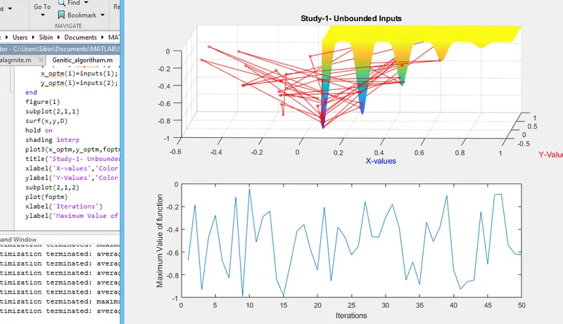
• Output shown below

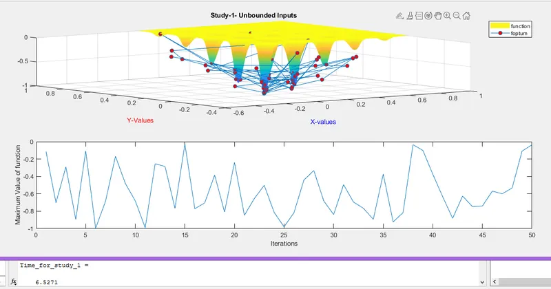
• As we know the GA predict actualy the minimum value of the function, but due to putting a -ve sign in the stalagmite function equation during the creation of the function stalagmite.m, the value obtained here are maximum values of the function (take only modulus values).
• Here the colored surface shows the stalagmite function and the red dots shows the maximum value of the functions obtained after completeing the Genetic algorithm function 50 iterations. The sub plot gives the variation in the maximum values of function during the 50 iterations.
• The plot indicate lot of local maximum values (modulus of the value indicated in the plot, because we put a -ve sign in the stalagmite function equation). But it shows lot of local maximaes and we cannot identify the global maxima. So the result of the study-1 doesnot provide the solution we want. so we do 2nd study by giving bounded conditions.
• Here the maximum value is between the 0 and -1 as shown in the subplot between the maximum value of the function and no.of iterations.
• It takes 6.5271 sec to complete the 1st study.

Study-2 Bounded inputs by setting the Upper and lower bounds

• The steps are same as that mentioned in the study-1. Only difference is in the syntax of GA function. Here we provided the bounded conditions/constraints that is the upper and lower limits between which the GA predicts the maximum value( Actualy minimum value,but here maximum value).
• Finds optimum values of the function and its coordinates and stored it in foptm and inputs (with boundary conditions).
• Setup bounds for the variables x and y of the function
• [inputs, foptm(i)]= ga(@stalagmite,2,[],[],[],[],[0;0],[1;1]); here the function predicts maximum value between the lower limit represented as [0;0] and upper limits represented as[1;1]. The other linear and non linear constraints are not exist so marked as [ ] in their respective places.
• Output is shown below

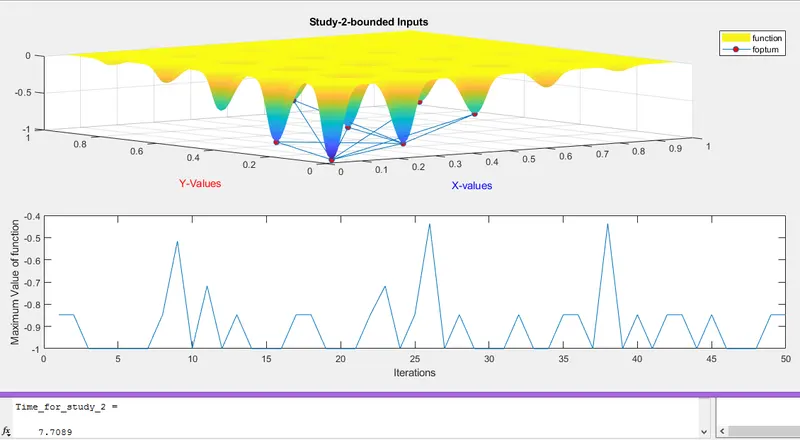
• Here as shown in the figure the no.of local maximas is reduced to fewer numbers between the upper and lower bounds.
• The function predicts maximum points lay between the 7 points and its optimum value is between -0.4 and -1 as shown in the plot between the maximum value of the function and no.of iterations.
• It takes 7.7089 sec to complete the 2nd study.

Study-3 bounded inputs(upper and lower limits) with incresed population size

• The steps are same as that mentioned in the study-1 and 2, the difference is that inadition to specifing the bounds change the initial population size.
• In GA normaly it starts with random samples, so by default it takes 50 as the sample size. Since there are 2 variables there is 50 sets of 2 random variables and takes it as initial population.
• If the initial population size is too small it can't find global minima(here maxima) instead it finds the local minimas.
• So inorder to avoid that and to find the global maxima increased the population size to 300. but the it affect the speed of exicution of GA, ie it slow down the GA and takes long simulation time.
• The modifictions in the population size is done by using the command "options = optimoptions(SolverName,Name,Value)" it returns options with specified parameters set using one or more name-value pair arguments. eg; option=optimoptions("ga");
  option=optimoptions(option,'PopulationSize',300);
• Here the GA syntax is represented inside the for loop as [inputs, foptm(i)]=ga(@stalagmite,2,[],[],[],[],[0;0],[1;1],[],[],option); the "option" in the syntax represent the modified population size as 300.
• Output is given below

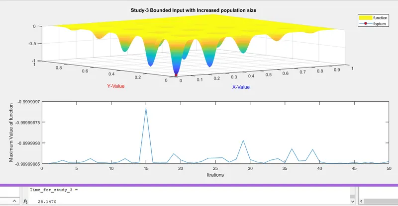
• Here it shows only one optimum point whchi we wanted as result.
• Also the Maximum value of function vs No. of Iterations gives the range of maximum value is between the -0.9999997 and -0.99999985
• So we find the Global maxima as almost equal to 1(|-1|).
• As the initial population size is changed to 300 it takes 28.147 sec to complete the study-3.

Errors and Problems Faced

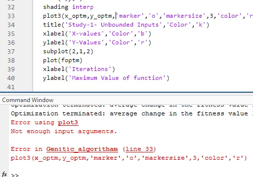
• Error occured due to lack of providing enough input arguments in the plot command. Here the "foptm" value is not provided in the plot3 command
• Rectified by providing the required input arguments.

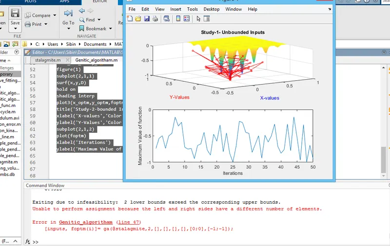
• Error due to putting the upper bounds lower than the lower bounds in the GA syntax.
• The lower bounds provided exceeds the corresponding upper bounds.
• Corrected by providing upper bound greater than lower bound.

• The stalagmite function is correctly displayed in the plot.
• It is due to the problem in the stalagmite function equation. In the final equation it lacks the -ve sign. rectified by providing the required equations.

Error

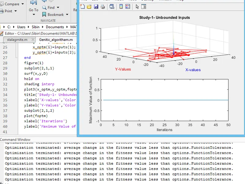
Error Corrected

Conclusion

• The code in MATLAB to optimise the stalagmite function written and exicuted successfully.
• The 3 studies helps to understand and visualize how the GA and its algorithm works and produce the required result we looking for.
• After the 3 studies we could findout the global maxima of the function.

References

1. https://in.mathworks.com/help/gads/ga.html?searchHighlight=ga&s_tid=srchtitle
2. https://in.mathworks.com/help/optim/ug/optim.problemdef.optimizationproblem.optimoptions.html
3. https://en.wikipedia.org/wiki/Genetic_algorithm
4. https://towardsdatascience.com/introduction-to-genetic-algorithms-including-example-code-e396e98d8bf3#:~:text=A%20genetic%20algorithm%20is%20a,offspring%20of%20the%20next%20generation.