Week 3 - Solving second order ODEs

Aim

Write a program that solves the following ODE `(d^2theta)/dt^2+b/m*(d theta)/dt+g/L*sintheta=0` that represents the equation of motion of a simple pendulum with damping.

Objectives

• Write a program that solves the following ODE `(d^2theta)/dt^2+b/m*(d theta)/dt+g/L*sintheta=0` that represents the equation of motion of a simple pendulum with damping.

• In the above equation,

  g = 9.81 (gravity in m/s2)

  L = 1 (length of the pendulum in m)

  m = 1 (mass of the ball in kg)

  b= 0.05 (damping coefficient)

• Write a program in Matlab\Octave that will simulate the pendulum motion between 0-20 sec, for angular displacement=0, angular velocity=3 rad/sec at time t=0.
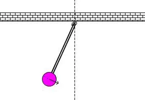
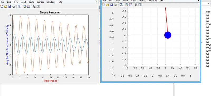
• Use this information to animate the motion of the pendulum, as shown in the below figure.

Methodology

Theory and Governing Equations

In Engineering, ODE is used to describe the transient behavior of a system. A simple example is a pendulum. The way the pendulum moves depends on the Newtons second law. When this law is written down, we get a second order Ordinary Differential Equation that describes the position of the "ball" w.r.t time. Similarly, there are hundreds of ODEs that describe key phenomena like motion of spring mass and damper system, mechanical vibration applications etc.

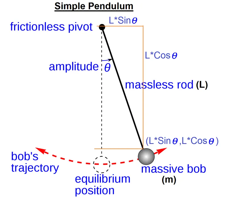
A simple pendulum consist of a small diameter bob of mass m and an inextensible string of negligible mass. Its one end attached to the bob and other is pivoted at a point which allow it free to move. When a pendulum is displaced sideways from its resting or equlibrium position, the restoring force created in it due to the gravity accelerate it towards the equilibrium position and make a to and fro motion and finaly come to rest. This oscillation of bob about equlibrium position is a simple harmonic motion. The time for one complete cycle, a left swing and a right swing, is called the period of oscillation and it depends on the length of the string hanging the bob.

The Time period of Pendulum is given as,

`T=2pisqrt(L/g)`

L is the length of pendulum and g is the acceleration due to gravity.

Equation of Motion of Pendulum

`(d^2theta)/dt^2+b/m*(d theta)/dt+g/L*sintheta=0`

This should be changed to first order ordinary differential equation(ODE) inorder to solve the equation. for that

put `theta=theta_1`

differentiating `theta` with respect to t we get `theta_2`

`(d theta)/dt=(d theta_1)/dt=theta_2` ---------- 1

differentiating further gives

`(d^2theta)/dt^2=(d^2theta_1)/dt^2=d/dt((d theta_1)/dt)=(d theta_2)/dt` -----------2

putting equation 1 and 2 in the main ODE equation finaly we get

`(d theta_1)/dt=theta_2` and `(d theta_2)/dt=-b/m*theta_2-g/L*sintheta_1`

converting it into a column vector

`d/dt [[theta_1],[theta_2]]=[[theta_2],[-b/m*theta_2-g/L*sintheta_1]]`

final solution can be represented as

`d/dt[theta]=d/dt [[theta_1],[theta_2]]`

`[theta]=[[theta_1],[theta_2]]`

here `theta_1` represent the Angular displacement and `theta_2` represent angular velocity corrosponding to a time t.

Inputs Given

1. g = 9.81 (gravity in m/s2)
2. L = 1 (length of the pendulum in m)
3. m = 1 (mass of the ball in kg)
4. b= 0.05 (damping coefficient)
5. `theta=theta_1=` Angular Displacement
6. time period (t_span) - from t=0 sec to t=20 sec with 500 intervel points
7. Initial conditions - `theta_0`=[0,3], here it represent at time t=0, angular displacement `theta_(1_0)`=0 rad and Angular velocity `theta_(2_0)` = 3 rad/sec

Code Explanation

• provide the inputs given as above, b=0.05; g=9.81; m=1; l=1;
• provide the initial condition as "theta_0=[0;3];"
• provide the time period "t_span=linspace(0,20,500);"

Function Code "ode_func.m"

• A separate function named "ode_func.m" is created for arranging the first order ODE for solving it using the "ode45" ODE solver command in MATLAB. Here the function ode_func.m form the ODE "dtheta_dt" `((d theta)/dt)` which is defined inside the function
• `theta` is the column vector defiened as `[theta]=[[theta_1],[theta_2]]`
• After this we get the values for "dtheta1_dt" `((d theta_1)/dt)` and "dtheta2_dt `((d theta_2)/dt)`
• % creating a function to solve ODE and find angular velocity and
  % angular displacement along with ode45 ODE solver.
  function [dtheta_dt]=ode_func(t,theta,b,g,l,m)
  theta1=theta(1);
  theta2=theta(2);
  dtheta1_dt=theta2;
  dtheta2_dt=-(b/m)*theta2-(g/l)*sin(theta1);
  dtheta_dt=[dtheta1_dt;dtheta2_dt];
  end

ODE Solver "ode45"

• "ode45" is the ODE solver that helps to solve the nonstiff differential equations by integrating it within a certain limits and initial conditions.
• Here "ode45" solves this first order ODE and finds the values of `theta_1 and theta_2` for the time period (t_span) t=0 sec to t=20 sec with 500 intervels and initial condition "theta_0=[0;3]" from the "dtheta1_dt" `((d theta_1)/dt)` and "dtheta2_dt" `((d theta_2)/dt)` in the function by integrating it.
• The values of `theta_1 and theta_2`stored in the "results" vector having 500 rows and 2 columns.
• First column is the value of angular displacement `theta_1` and 2nd column is the Angular velocity `theta_2` with respect to the corresponding time points which is stored in the column vector "t".
• % solveing ODE using the ode45 command
  % separate function ode_func.m created for solving the ODE along with the
  % ode45 command
  [t,results]= ode45(@(t,theta)ode_func(t,theta,b,g,l,m),t_span,theta_0)

"For loop" to Creat animation

• pivoting point of pendulum is assigned as (x0,y0)=(0,0)
• access the 1st column of the results vector which is angular displacement and assigned to D "D=results(:,1);"
• "For" loop is used from i=1:length(t_span), t_span is the time points during which angular displacement and velocity are calculated. ie from t=0 to t=20 sec with 500 intervels.
• For each value of time point correcponding angular displacement is assigned to the variable A
  "A=D(i);"
• Coordinates of the pendulum is calculated using the angular displacement. since it is fixed on point (0,0) y-coordinate is -ve.
  x1=l*sin(A);
  y1=-l*cos(A);
• For each time value image is stored in the array M.
• After complete the 500 runs of "For" loop animation is created using code "Movie(M)"
• After that created a video file named "pendulum.avi" and open it and write the animation in it and close it.

for i=1:length(t_span)

A=D(i);

x1=l*sin(A);
y1=-l*cos(A);

figure(2)
plot([x0 x1],[y0 y1],'linewidth',2,'Color','r')
hold on
plot(x0,y0,'Marker','v','MarkerEdgeColor','g','MarkerSize',10,'MarkerFaceColor','b')
plot(x1,y1,'Marker','o','MarkerSize',30,'MarkerFaceColor','b','MarkerEdgeColor','r')
hold off
axis([-1 1 -2 0])
grid on

M(ct)=getframe(gcf);
ct=ct+1;
end

movie(M)

Pendulum=VideoWriter('pendulum.avi','Uncompressed AVI');

open(Pendulum)
writeVideo(Pendulum,M)
close(Pendulum)

MATLAB Program

Function Program

% creating a function to solve ODE and find angular velocity and
% angular displacement along with ode45 ODE solver.

function [dtheta_dt]=ode_func(t,theta,b,g,l,m)
         theta1=theta(1);
         theta2=theta(2);
         dtheta1_dt=theta2;
         dtheta2_dt=-(b/m)*theta2-(g/l)*sin(theta1);
         dtheta_dt=[dtheta1_dt;dtheta2_dt];
     end

Main Program

  
% Write a program that solves the first order ODE  
% that  represents the equation of motion of a simple pendulum with damping.

clear all
close all
clc

% Inputs
% damping constant
b=0.05;

% accelaretion due to gravity in m/s^2
g=9.81;

% mass of pendulum in kg
m=1;

% length of pendulum in m
l=1;

% initial condition
% displacement and velocity, column matrix
% ie for time t=0, displacement=0 and velocity=5rad/s
theta_0=[0;3];

% time period during which ODE is solved and displacement and velocity are calculated
% calculated for 500 values in between 0 and 10 seconds
t_span=linspace(0,20,500);

% solveing ODE using the ode45 command 
% separate function ode_func.m created for solving the ODE along with the
% ode45 command
[t,results]= ode45(@(t,theta)ode_func(t,theta,b,g,l,m),t_span,theta_0);

% all the values in the 1st column of the results array(displacement) stored in the array
% named D for plotting the position of pendulum at different angular
% displacement
D=results(:,1);

% plotting the angular displacement and angular velocity graph with respect
% to time period
figure(1)
plot(t,results(:,1))
hold on
plot(t,results(:,2))
title('Simple Pendulum','Color','k')
xlabel('Time Period','Color','r')
ylabel('Angular Displacement and Velocity','Color','b')

% pivoting point of simple pendulum
x0=0;
y0=0;
ct=1;

% Creating animation of simple pendulum
for i=1:length(t_span)

    % for each value of time point correcponding angular displacement is assigned
    % to the variable A
    A=D(i);

    % Coordinates of the pendulum is calculated using the angular
    % displacement
    x1=l*sin(A);
    y1=-l*cos(A);

    % plotting the pendulum traceout points, pivot point and pendulum bob
    figure(2)
    plot([x0 x1],[y0 y1],'linewidth',2,'Color','r')
    hold on
    plot(x0,y0,'Marker','v','MarkerEdgeColor','g','MarkerSize',10,'MarkerFaceColor','b')
    plot(x1,y1,'Marker','o','MarkerSize',30,'MarkerFaceColor','b','MarkerEdgeColor','r')
    hold off
    axis([-1 1 -2 0])
    grid on
    
    % creating animation by assigning each frame to M
    M(ct)=getframe(gcf);
    ct=ct+1;
end

% creating a movie by matlab using frames stored in M
movie(M)

% creating a video file "pendulum.avi" assigned to pendulum
Pendulum=VideoWriter('pendulum.avi','Uncompressed AVI');

% open the created file to write the video from M
open(Pendulum)
writeVideo(Pendulum,M)
close(Pendulum)

Errors and problems faced and Steps taken to overcome those

• Problem occured due to the lack of "hold off" command at the end of the plot command. Corrected by providing it at proper position.

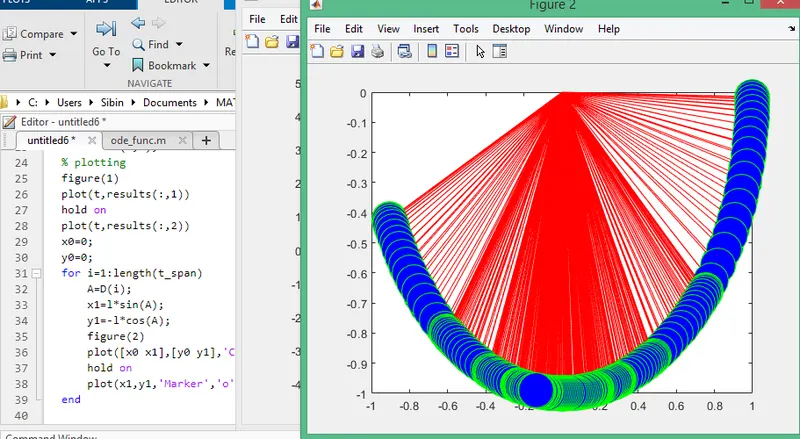
• Problem of changeing the x-axis as the pendulum swings.
• It is due to the lack of fixed axis limit and lack of placeing the axis limit code after the "hold on" command.
• Corrected by providing "axis([-1 1 -2 0])" at correct position.

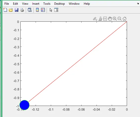
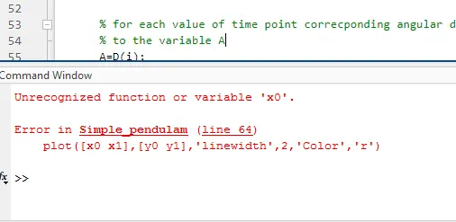
• Error occured due to not defining the variable x0 and y0 which is the pivoting point of pendulum.
• Corrected by putting x0=0 and y0=0 as pivot point of pendulum.

Final Output

Conclusion

• The program that solves the following ODE `(d^2theta)/dt^2+b/m*(d theta)/dt+g/L*sintheta=0` that represents the equation of motion of a simple pendulum with damping exicuted successfully.
• It helps in understanding the solving of first order ODE using function and "ode45", a versatile ODE solver in MATLAB
• The animation of the pendulam is done using the obtained solution and it works correctly hence concluded that the solution obtained by the program is correct.

Links are attached along with this report.

Youtube Link - https://youtu.be/-Ew2vmn5ly0

Google drive link - https://drive.google.com/file/d/1eX4HfdV31_YJTMqqiy0pMH9STFS4ZwJq/view?usp=sharing