Week 4.1 - Genetic Algorithm
AIM:
To write the code to calculate the global maxima of the stalagmite function and to explain the syntax for genetic algorithm(ga) in MATLAB.
OBJECTIVE:
- To write a code in MATLAB to optimize the stalagmite function and find global maxima of the function.
- To explain the concept of genetic algorithm and the syntax for ga in MATLAB.
- To plot the graph of all three studies and also for global maxima.
THEORY:
Stalagmite
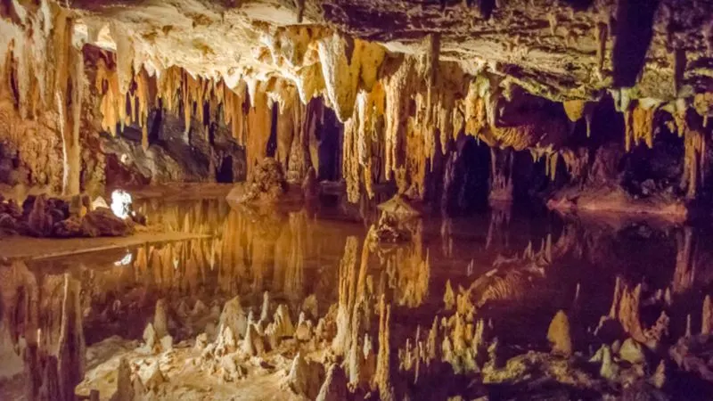
A stalagmite is a type of rock formation that rises from the floor of a cave to the accumulation of material deposited on the floor from ceiling drippings. Stalagmites are typically composed of calcium carbonate, but may consist of lava, mud, peat, pitch, sand, sinter and amberat.That is why we are using the stalagmite as the name for the program due to its shape
Genetic Algorithm(ga)
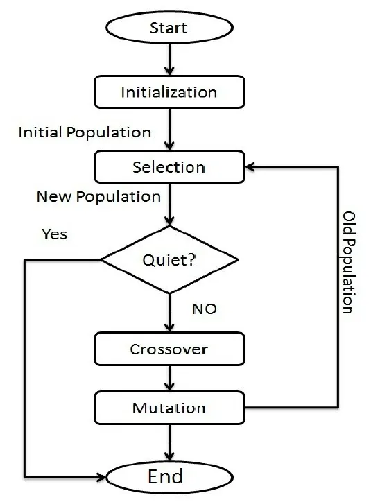
Genetic Algorithm(ga) is a search-based optimization technique based on the principles of Genetics and Natural Selection. It is frequently used to find optimal or near-optimal solutions to difficult problems which otherwise would take a lifetime to solve. It is frequently used to solve optimization problems, in research, and in machine learning.
Mathematical Equations:
To find global maxima
f= (f1 . f2 . f3 . f4)
To find global maxima
f = - (f1 . f2 . f3 . f4)
Where
f1 = [sin(5.1pax + 0.5)]^6
f2 = [sin(5.1pay + 0.5)]^6
f3 = exp(- 4 * log (2) * (x - 0.0667) ^ 2/0.64)
f4 = exp(- 4 *log (2) * (y - 0.0667) ^ 2/0.64)
Here x and y are two variables.
PROGRAM:
For plotting Global Maxima
clear all

close all

clc


% defining the our search space

x = linspace(0,0.6,150);

y = linspace(0,0.6,150);

num_cases=50


% Creating a 2Dimensional mesh

[xx yy] = meshgrid(x, y);


%Evaluating the stalagmite function

for i = 1:length(xx)

    for j = 1:length(yy)

        input_vector(1) = xx(i,j);

        input_vector(2) = yy(i,j);

        f(i,j) = stalagmite(input_vector);

    end

end


surfc(xx,yy,f)

xlabel('x value')

ylabel('y value')

shading interp

[inputs,fval] = ga(@stalagmite,2)
Function:
function [f] = stalagmite(input_vector)


x = input_vector(1);

y = input_vector(2);

f1 = (sin(5.1*pi*x+0.5))^6;

f2 = (sin(5.1*pi*y+0.5))^6;

f3 = exp(-4*log(2)*(x-0.0667)^2/0.64);

f4 = exp(-4*log(2)*(y-0.0667)^2/0.64);


f = (f1*f2*f3*f4);

end
Here for plotting global minima and finding the minimum of the function ga is used
clear all

close all

clc


% defining the our search space

x = linspace(0,0.6,150);

y = linspace(0,0.6,150);

num_cases=50


% Creating a 2Dimensional mesh

[xx yy] = meshgrid(x, y);


%Evaluating the stalagmite function

for i = 1:length(xx)

    for j = 1:length(yy)

        input_vector(1) = xx(i,j);

        input_vector(2) = yy(i,j);

        f(i,j) = stalagmite(input_vector);

    end

end


for i=1:num_cases

[inputs,fopt(i)] = ga(@get_stalagmite, 2);

xopt(i) = inputs(1);

yopt(i) = inputs(2);

end


figure(1)

subplot(2,1,1)

surface(x,y,f)

hold on

xlabel('x value')

ylabel('y value')

shading interp

[inputs,fval]=ga(@get_stalagmite,2)

plot3(xopt,yopt,fopt,'marker','o','markersize',3,'markerfacecolor','g')

subplot(2,1,2)

plot(fopt)

xlabel('iterations')

ylabel('Function Minimum')


tic


 %Study 2-Boundary Limits


for i =1:num_cases

    [inputs,fopt(i)] = ga(@get_stalagmite,2,[],[],[],[],[0;0],[0.6;0.6]);

    xopt(i) = inputs(1);

    yopt(i) = inputs(2);

end


study2_time = toc;


%plotting2

figure(2)

subplot(2,1,1)

hold on

surfc(x,y,f)

shading interp

plot3(xopt,yopt,fopt,'marker','o','markersize',3,'markerfacecolor','g')

title('Bounded inputs')

subplot(2,1,2)

plot(fopt)

xlabel('iterations')

ylabel('Function Minimum')


% increasing ga iteration

options = optimoptions('ga');

options = optimoptions(options,'populationsize',180);


tic


for i =1:num_cases

    [inputs,fopt(i)] = ga(@get_stalagmite,2,[],[],[],[],[0;0],[0.6;0.6],[],[],options);

    xopt(i) = inputs(1);

    yopt(i) = inputs(2);

end


study3_time = toc;


%plotting3

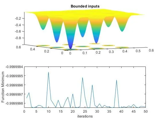
figure(3)

subplot(2,1,1)

hold on

surfc(x,y,f)

shading interp

plot3(xopt,yopt,fopt,'marker','o','markersize',5,'markerfacecolor','g')

title('Bounded inputs')

subplot(2,1,2)

plot(fopt)

xlabel('iterations')

ylabel('Function Minimum')
Function
function[f]=get_stalagmite(input_vector)


x = input_vector(1);

y = input_vector(2);

f1 = (sin(5.1*pi*x+0.5))^6;

f2 = (sin(5.1*pi*y+0.5))^6;

f3 = exp(-4*log(2)*(x-0.0667)^2/0.64);

f4 = exp(-4*log(2)*(y-0.0667)^2/0.64);


f = -(f1*f2*f3*f4);

end
OUTPUTS:
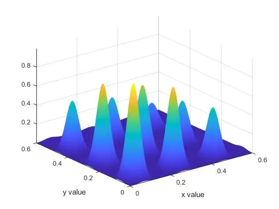
For global maxima
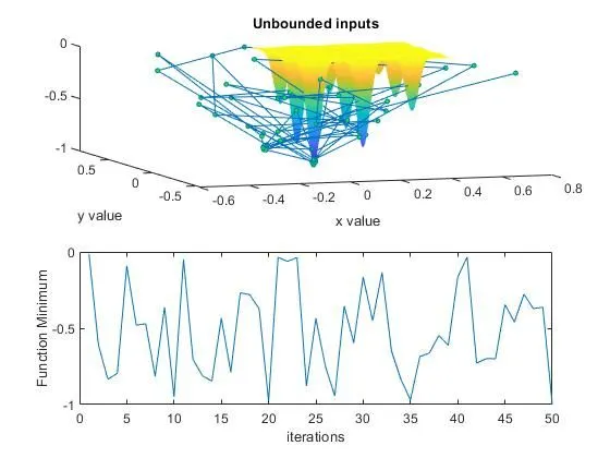
For finding minimum function by ga study1
For finding minimum function by ga study2
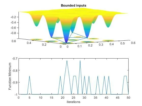
For finding minimum function by ga study2
RESULT:
- The code for global maxima and stalagmite function is done.
- The concept of genetic algoritham and the syntax is done.
- The graph for all three studies and global maxima are plotted.