Week 3 - Solving second order ODEs

AIM:

       ‘Solving Second Order Equation’.

OBJECTIVE:

• Write a program in Matlab/Octave that will simulate the pendulum motion.
• Write a program that solves the following ODE. This ODE represents the equation of motion of a simple pendulum with damping.

THEORY:

    1.What is a Simple Pendulum?

         A simple pendulum is a weight suspended from a pivot so that it can swing freely.When a pendulum is displaced sideways from its resting, equilibrium position, it is subject to a restoring force due to gravity that will accelerate it back toward the equilibrium position.

                                         

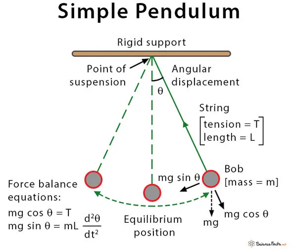
    2.Theory Of Simple Pendulum:

         A simple pendulum consists of a mass m hanging at the end of string of length L. The period of a pendulum or any oscillatory motion is the time required for one complete cycle, that is, the time to go back and forth once.

    3.Governing Equation:

        Second-order ODE representing the equation of a simple pendulum motion.

              In the above equation,

                        g = gravity in m/s2,

                        L = length of the pendulum im m,

                        m = mass of the ball in kg,

                        b = damping coefficient,

                        To write a program in matlab/octave that will simulate the pendulum motion, just like the one shown in the start of this challenge

                        We are using,

                        L = 1m,

                        m = 1kg,

                        b = 0.05,

                        g = 9.81m/s2.

MATLAB PROGRAM CODE:

clear all

close all

clc



% inputs

l = 1;

m = 1;

b = 0.05;

g = 9.81;



% initial condition

theta_0 = [0;5];



% time points

t_span = linspace(0,100,500);



% solve ODE

[t,results] = ode45(@(t,theta) ode_func(t,theta,b,g,l,m),t_span, theta_0);



% plot

figure(1)

plot(t,results(:,1))

hold on

plot(t,results(:,2))

xlabel('Position-Radians')

ylabel('Angular Velocity')

title("Displacement vs Velocity")

legend('Displacement','Velocity')




% for loop

ct = 1;

for a =1:length(results(:,1))

    x1 = -1*sind(results(a,1));

    y1 = -1*cosd(results(a,1));

    

    figure(2)

    plot([0,x1],[0,y1],'linewidth',1)

    hold on

    plot(x1,y1,'o','color','r')

    hold off

    axis([-.2,.2,-1.1,0])

    pause(.006)

    

    % storing frames in m

    M(ct) = getframe(gcf);

    ct = ct+1;

end




% Creating videofile for m

movie(M)

videofile = VideoWriter('forwardkinematics.avi','uncompressed AVI');

open(videofile);

writeVideo(videofile,M);

close(videofile)

MATLAB CODE FUNCTION OF ‘ode.m’:

function [dtheta_dt] = ode_func(t,theta,b,g,l,m)

         theta1 = theta(1);

         theta2 = theta(2);

         dtheta1_dt = theta2;

         dtheta2_dt = -(b/m)*theta2  - (g/l)*sind(theta1);

         dtheta_dt = [dtheta1_dt; dtheta2_dt];

end  

RESULTS:

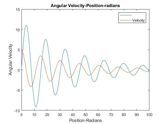
       For better understanding, I am providing time = 100secs

         Plot Diagram: From the plot we can clearly see that as the damping coefficient increases the damping effect also                                                                        increases that means there will be less oscilations.

             

           Animation Video link:

                https://drive.google.com/file/d/1BNq7XwKvhl1D4g7O0hnwEZBeOt66WVGs/view?usp=sharing