Project 2 - Rankine cycle Simulator

Aim:-

The aim of the project is to simulate the Rankine Cycle for the inputs provided by user

Theory:-

The Rankine Cycle is basic thermodynamic cycle that converts heat energy into mechanical energy

It consist of 4 process

1. 1-2 is isentropic expansion in the turbine
2. 2-3 is constant pressure heat removal in the condenser
3. 3-4 is the isentropic compression in the pump
4. 4-1 is the constant pressure heat addition in the boiler

The Efficiency of this cycle is given by

Eff = Wnet/Qin*100

The Back Work Ratio is given by

BWR = Wp/Wt(Work Done on pump/work done by turbine)

To calculate the state point we will use the given steam table (XSteam)

Procedure:-

To start with we need the input from the user so we use ‘fprintf’ to show what we need to display in the command window and ‘input’ command to take the input the given by user

Then we calculate all the state point variable with the help of XSteam Function provided

Now after calculating the entire state variable we need to calculate the Thermal Efficiency and Back Work Ratio for which we need to calculate

• Work done by turbine (Wt)
• Work done on pump (Wp)
• Net work done (Wnet)
• Heat out of the system (Qout)
• Heat into the system (Qin)

With the help of above elements we can calculate the efficiency and back work ratio

The Efficiency of this cycle is given by

Eff = Wnet/Qin*100

The Back Work Ratio is given by

BWR = Wp/Wt(Work Done on pump/work done by turbine)

Now we can plot the T-S & H-S Diagram as we have all the state variables for which we will use ‘Plot’ Command and we save both the curves in 2 figures (figure(1) & figure(2).

And we label the axis & Title accordingly

Main Code

clear all
close all
clc

disp('RANKINE CYCLE');
disp('1-2 is isentropic expansion in the turbine');
disp('2-3 is constant pressure heat removal in the condensor');
disp('3-4 is the isentropic compression in the pump');
disp('4-1 is the constant pressure heat addition in the boiler');

%taking inputs from user
p1 = input('Value of pressure at inlet turbine, p1(bar)= ');
t1 = input('Value of temperature at inlet turbine, t1(celsius)= ');
p2 = input('Value of pressure at inlet condensor, p2(bar)= ');

%calulating the state variables

%state point1

h1 = XSteam('h_pt',p1,t1);
s1 = XSteam('s_pt',p1,t1);

%state point 2 

s2 = s1;
hf2 = XSteam('hL_p',p2);
hg2 = XSteam('hV_p',p2);
sf2 = XSteam('sL_p',p2);
sg2 = XSteam('sV_p',p2);
x2 = (s2-sf2)/(sg2-sf2);
h2 = hf2 + (x2*(hg2-hf2));
t2 = XSteam('Tsat_p', p2);

%state point 3

p3 = p2;
h3 = XSteam('hL_p',p3);
s3 = XSteam('sL_p',p2);
t3 = t2;
v3 = XSteam('vL_p',p3);

%state point 4

p4 = p1;
s4 = s3;

%work done on pump

Wp = (v3*(p4-p3))*100;

h4 = h3 + Wp;
cp4 = XSteam('Cp_ps',p4,s4);
cv4 = XSteam('Cv_ps',p4,s4);
k = cp4/cv4;
t4 = t3/((p3/p4)^((k-1)/k));

%work done

%work done by turbine

Wt = h1-h2;

%net work done

Wnet = Wt-Wp;

% heat into the system

Qin = h1-h4;

% heat out of the system

Qout = h2-h3;

%thermal efficiency

Eff = (Wnet/Qin)*100;

% Specific Steam Consumption
%SSC = mass flow rate/power
SSC = 3600/Wnet;

% back work ratio
BWR = (h4-h3)/(h1-h2);

% calculating the temprature enthalpy & entropy at liquid and vapuor state

t5 = XSteam('Tsat_p',p1);
s5 = XSteam('sL_p',p1);
h5 = XSteam('hL_p',p1);
t6 = t5;
s6 = XSteam('sV_p',p1);
h6 = XSteam('hV_p',p1);

% printing all state variables
fprintf('\n--------RESULT---------\n')
fprintf('At state point 1:\n P1 is : %4.2f Bar\n T1 is : %4.2f Degree Celsius\n H1 is : %4.2f Kj/kg\n S1 is : %4.2f Kj/KgK\n\n',p1,t1,h1,s1)
fprintf('At state point 2:\n P2 is : %4.2f Bar\n T2 is : %4.2f Degree Celsius\n H2 is : %4.2f Kj/kg\n S2 is : %4.2f Kj/KgK\n\n',p1,t1,h1,s1)
fprintf('At state point 3:\n P3 is : %4.2f Bar\n T3 is : %4.2f Degree Celsius\n H3 is : %4.2f Kj/kg\n S3 is : %4.2f Kj/KgK\n\n',p1,t1,h1,s1)
fprintf('At state point 4:\n P4 is : %4.2f Bar\n T4 is : %4.2f Degree Celsius\n H4 is : %4.2f Kj/kg\n S4 is : %4.2f Kj/KgK\n\n',p1,t1,h1,s1)
fprintf('Wt is : %4.2f Kj/Kg \n Wp is : %4.2f Kj/Kg \nWnet is : %4.2f Kj/Kg \nSSC is : %4.2f Kg/KWh \nThermal Efficiency is : %4.2f Percent \nBack Work Ratio is : %4.10f',Wt,Wp,Wnet,SSC,Eff,BWR)



% plotting the curve

t = linspace(1,400,1000);
for i = 1:length(t)
    sf(i)=XSteam('sL_T',t(i));
    sg(i)=XSteam('sV_T',t(i));
    hf(i)=XSteam('hL_t',t(i));
    hg(i)=XSteam('hV_T',t(i));

end

T_Rankine = linspace(t5,t1,5000);
for j = 1:length(T_Rankine)
    S_Rankine(j)=XSteam('s_pT',p1,T_Rankine(j));
end

% plotting t-s curve

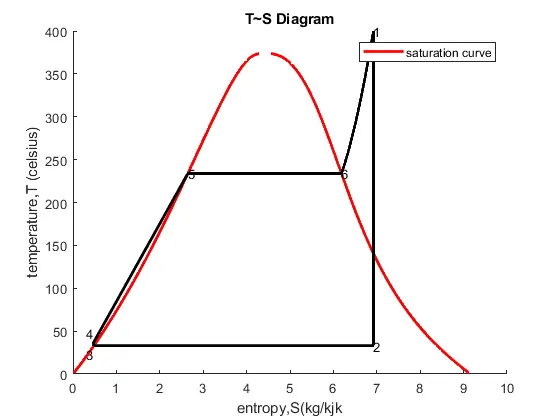
figure(1)
hold on
plot(sf,t,'r','LineWidth',2);
plot(sg,t,'r','LineWidth',2);
plot([s1 s2 s3 s4 s5 s6 S_Rankine],[t1 t2 t3 t4 t5 t6 T_Rankine], 'k', 'LineWidth',2);

text(s1,t1,'1')
text(s2,t2,'2')
text(s3,t3,'3','VerticalAlignment','top','HorizontalAlignment','right')
text(s4,t4,'4','VerticalAlignment','bottom','HorizontalAlignment','right')
text(s5,t5,'5')
text(s6,t6,'6')

title('T~S Diagram');
xlabel('entropy,S(kg/kjk');
ylabel('temperature,T (celsius)');
legend('saturation curve');

%ploting h-s curve
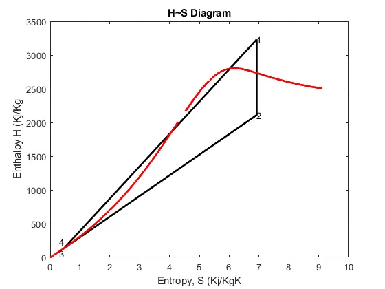
figure(2)
plot([s1 s2 s3 s4 s1],[h1 h2 h3 h4 h1],'k','LineWidth',2);
hold on
plot(sg,hg,'r','LineWidth',2);
plot(sf,hf,'r','LineWidth',2);


text(s1,h1,'1')
text(s2,h2,'2')
text(s3,h3,'3','HorizontalAlignment','right','VerticalAlignment','top')
text(s4,h4,'4','HorizontalAlignment','right','VerticalAlignment','bottom')

xlabel('Entropy, S (Kj/KgK');
ylabel('Enthalpy H (Kj/Kg');
title('H~S Diagram')

Command Window

RANKINE CYCLE
1-2 is isentropic expansion in the turbine
2-3 is constant pressure heat removal in the condensor
3-4 is the isentropic compression in the pump
4-1 is the constant pressure heat addition in the boiler
Value of pressure at inlet turbine, p1(bar)= 30
Value of temperature at inlet turbine, t1(celsius)= 400
Value of pressure at inlet condensor, p2(bar)= 0.05

--------RESULT---------
At state point 1:
 P1 is : 30.00 Bar
 T1 is : 400.00 Degree Celsius
 H1 is : 3231.57 Kj/kg
 S1 is : 6.92 Kj/KgK

At state point 2:
 P2 is : 30.00 Bar
 T2 is : 400.00 Degree Celsius
 H2 is : 3231.57 Kj/kg
 S2 is : 6.92 Kj/KgK

At state point 3:
 P3 is : 30.00 Bar
 T3 is : 400.00 Degree Celsius
 H3 is : 3231.57 Kj/kg
 S3 is : 6.92 Kj/KgK

At state point 4:
 P4 is : 30.00 Bar
 T4 is : 400.00 Degree Celsius
 H4 is : 3231.57 Kj/kg
 S4 is : 6.92 Kj/KgK

Wt is : 1120.86 Kj/Kg 
 Wp is : 3.01 Kj/Kg 
Wnet is : 1117.85 Kj/Kg 
SSC is : 3.22 Kg/KWh 
Thermal Efficiency is : 36.17 Percent 
Back Work Ratio is : 0.0026862672>> 

Conclusion

Thermal Efficiency of the Rankine Cycle is :- 36.17%

Back Work Ratio of Rankine Cycle is :- 0.0026862672

T-S Diagram

H-S Diagram

Error During Compilation

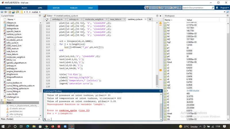
typing Error in length command