Week 4.1 - Genetic Algorithm
Aim: To develop programs to solve genetic algorithm and different cases of it moreover, to study and understand principle and process of GA.
Principle: The Genetic Algorithm is a well-known metaheuristic stochastic optimization algorithm based on Charles Darwin's theory of natural evolution's natural selection mechanisms. An example of mechanism is shown in figure (1) and its step wise process is explained.
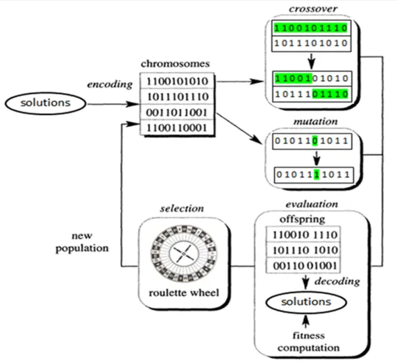
Figure (1) Gentetic Algorithm Process
- A genetic algorithm begins with a population of random solutions.
- Each member in the population is referred to as a chromosome, and each chromosome represents a solution to the problem at hand.
- The chromosomes change with period in iterations known as generations.
- The fitness of the chromosomes is assessed at the end of each generation.
- New chromosomes, known as offspring, are generated by either (a) combining two chromosomes from the present generation using a crossover operator or (b) changing a chromosome using a mutation operator to establish the next generation.
- To maintain the population size constant, a new generation is generated by (a) selecting some of the parents and offspring based on fitness values and (b) rejecting others.
- Fitter chromosomes have a better chance of being chosen.
- The algorithms eventually settle on the best chromosome after numerous generations.
In most cases, GA maintains one of the following termination conditions:
When the population has not improved for several iterations.
When reaches a certain number of generations.
When the objective function value reaches a pre-defined threshold.
There might be several minima and maxima in a function. Global minima refer to the moment at which a function takes its smallest value. Local minima will be used to represent the remaining lower points. Similarly, global maxima refer to the point at which a function reaches its highest value. Local maxima will be used to represent the remaining higher points.
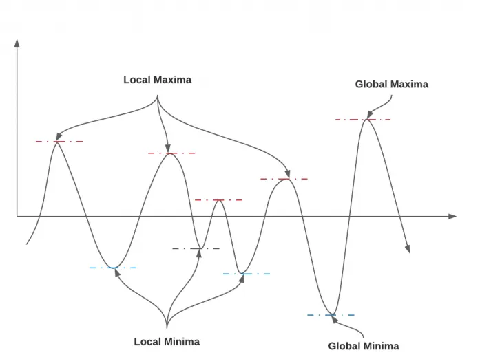
Figure (2) Maxima and Minima
Governing Equations: Stalagmite is a type of rock that is formed due to material deposition on floor or ceiling and its equation is given by
`f(x,y) = f1,x f2,xf1,yf2,y`
`f1x=[sin(5.1pix+0.5)]^6`
`f1y=[sin(5.1piy+0.5)]^6`
`f2x=exp[-4log(2)(x-0.0667)^2/0.64]`
`f2y=exp[-4log(2)(y-0.0667)^2/0.64]`
Coding: Coding section includes two programs such as main program and function program. The codes and explanations are given below.
Main Program: The program code is given below and each section is numbered inside brackets for explanation purpose. Program contains three case studies of GA 1. Unbounded inputs, 2. Bounded inputs and 3. Increased population size.
clear all
close all
clc

% Defining Search Space (1)
x = linspace(0,0.6,150);
y = linspace(0,0.6,150);

% Creating 2D mesh (2)
[xx yy] = meshgrid(x,y);

% Evaluating the Stalagmite Function
for i=1:length(xx)
    for j=1:length(yy)
        input_vector(1) = xx(i,j);
        input_vector(2) = yy(i,j);
        f(i,j) = stalagmite(input_vector);
    end
end

% Plotting Stalagmite Function(3)
figure(1)
surf(xx, yy , -(f))
shading interp
title('Stalagmite Function')
xlabel('X value')
ylabel('Y value')

% Case-1 Statistical behavior with unbounded inputs(4)
num_iter = 50;
tic
for i =1:num_iter
[inputs fopt(i)] = ga(@stalagmite, 2);
xopt(i) = inputs(1);
yopt(i) = inputs(2);
end
slove_time1 = toc % Measures elapsed time for case 1

% Plotting case-1 (5)
figure(2)
subplot(2,1,1)
hold on
surf(xx, yy , -(f))
shading interp
plot3(xopt,yopt,-fopt,'marker','o','markersize',5,'markerfacecolor','r')
title('Unbounded Inputs')
[subplot(2,1,2)]
plot(-fopt)
xlabel('iterations')
ylabel('function minimum')
zlabel('function Value')

% Case-2 Statistical behavior with upper and lower bands (6)
tic
for i =1:num_iter
[inputs, fopt(i)] = ga(@stalagmite,2,[],[],[],[],[0;0],[0.6;0.6]);
xopt(i) = inputs(1);
yopt(i) = inputs(2);
end
slove_time2 = toc % Measures elapsed time for case 2

% Plotting case-2 (7)
figure(3)
subplot(2,1,1)
hold on
surf(xx, yy , -(f))
shading interp
plot3(xopt,yopt,-fopt,'marker','o','markersize',5,'markerfacecolor','r')
title('Boundary Conditions')
[subplot(2,1,2)]
plot(-fopt)
xlabel('iterations')
ylabel('function minimum')
zlabel('function Value')


% Case-3 Statistical behavior with increased population size (8)
options = optimoptions('ga');
options = optimoptions(options,'populationsize',170);

tic
for i =1:num_iter
[inputs, fopt1(i)] = ga(@stalagmite,2,[],[],[],[],[0;0],[0.6;0.6],[],[],options);
xopt(i) = inputs(1);
yopt(i) = inputs(2);
end
slove_time3 = toc % Measures elapsed time for case 3

% Plotting case-3 (9)
figure(4)
subplot(2,1,1)
hold on
surf(xx, yy , -(f))
shading interp
plot3(xopt,yopt,-fopt1,'marker','o','markersize',5,'markerfacecolor','r')
title('Increased Population size')
[subplot(2,1,2)]
plot(-fopt1)
xlabel('iterations')
ylabel('function minimum')
zlabel('function Value')
G_max = max(abs(fopt1));
sprintf( 'Global maxima= %e', G_max)
Syntax of ga:Before Explaining Program syntax of ga needed to be explained. ga find the minimum of function.
- [x, fval] = ga(fun,nvars) - for any previous input arguments, also returns fval, the value of the fitness function at x.
For example in program [inputs, fopt] = ga(@stalagmite,2) -For previous input statements returns value of the fitness function (fopt) at inputs furthermore, finds a local unconstrained minimum inputs to the mentioned function (stalagmite). 2 is dimension of stalagmite function.
- [x, fval] = ga(fun,nvars,A,b,Aeq,beq,lb,ub,nonlcon,options) minimizes with the default optimization parameters replaced by values in options. Parameters and it's purpose of usage is given below.
fun- Calling function fun.
nvars- Dimension of function fun.
A, B – Linear inequalities, x subject to Linear inequalities A*x*<=B
Aeq, Beq - x subject to the linear equalities Aeq*x = beq and A*x ≤ b.
lb, ub – Defines set of lower and upper bound on design variables, x, so solution woll be in the range of lb<=x<=ub
nonlcon - The function nonlcon accepts x and returns vectors nonlinear inequalities and equalities (C and Ceq). ga minimizes the fun such that C(x) ≤ 0 and Ceq(x) = 0.
intcon – variable listed in intcon only take integer values.
Options- The default optimization settings are substituted by values in options to minimise, create options using optimoptions.
Set [] If there is no values for A,b,Aeq,beq,lb,uband nonlcon.
The explanation of sections in the program is given below.
Section (1) – for creating search space x and y are divided into 150 pieces between 0 to 0.6. Creating input array for x and y.
Section (2) – Creating 2d array using meshgird and each element in the array is stored input_vector variables with the help of for loop. Stalagmite function is called to determine each function value for corresponding elements.
Section (3) – A new figure window is used to plot three dimensional stalagmite functions and shading interp command is to avoid grid by putting shading effect.
Section (4) – 50 number of iterations is performed and for loop runs till last iterations. In every iterations loop evaluate stalagmite function value and returns to fopt variable additionally, xopt and yopt used to store x and y values.
Section (5) –A new figure is used to plot case 1 and two plots are accommodated inside a window using subplot. Second plot is to show optimum values of function in each iterations furthermore, graphs are labeled and titled with suitable names.
Section (6) – 50 number of iterations is assigned and for loop runs till last iterations. In every iteration loop evaluate stalagmite function value and returns to fopt variable additionally, boundary conditions (lb and ub) are applied. xopt and yopt used to store x and y values.
Section (7) – A new figure is used to plot case 2 and two plots are accommodated inside a window using subplot. Graphs are labeled and titled with suitable names.
Section (8) –Here population size is increased to 170 by utilizing options in ga function. In every iteration loop evaluate stalagmite function value and returns to fopt variable additionally, boundary conditions (lb and ub) are applied.
Section (9) – A new figure is used to plot case 3 and two plots are accommodated inside a window using subplot. Graphs are labelled and titled with suitable names. G_max variable gives maximum value in fopt1 that is global maxima value.
Function Program:
The program to create stalagmite function is shown below.
% stalagmite equation
function [v]= stalagmite(input_vector)
x = input_vector(1);
y = input_vector(2);
f1x = (sin(5.1*pi*x+0.5))^6;
f1y = (sin(5.1*pi*y+0.5))^6;
f2x = exp((-4*log(2)*(x-0.00667)^2)/.64);
f2y = exp((-4*log(2)*(y-0.00667)^2)/.64);
v = -(f1x*f2x*f1y*f2y);
end
Stalagmite named function is created with output variable v and input variable as input_vector. The given equation is implemented and assigned to v.
Outputs:
The figure (3) representing a stalagmite function 3D view.
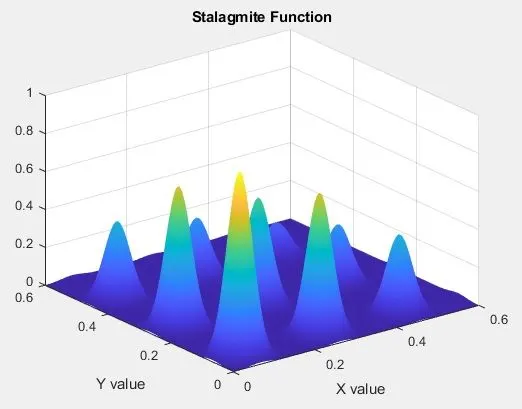
Figure (3) Stalagmite function 3D view
Case Study 1: Statistical behaviour with unbounded inputs result is shown in figure (4).
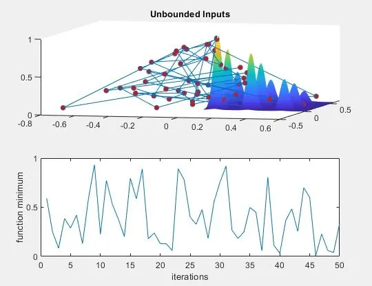
Figure (4) Case study 1
It is clear from the graph that the solution is not accurate it is lies between 0-1.The maxima values are in large range areas because of unbounded inputs. The ellapsed time for this case founded :study_time1 = 5.5814.
Case Study 2: Statistical behaviour with bounded inputs results is shown in figure (5).
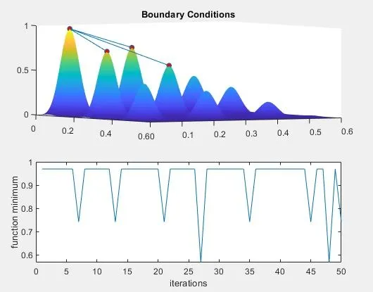
Figure (5) Case study 2
It is evident from the graph that the solution is not accurate however, better than previous case study and it is lies between 0.6-1. The maxima values are in small range area in comparison with unbounded inputs. The ellapsed time for this case founded :study_time2 = 7.8610.
Case Study 3: Statistical behaviour with bounded inputs and increased population size results is shown in figure (6).
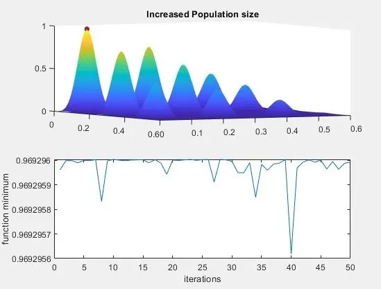
Figure (6) Case study 3
It is visible from the graph that the solution is much accurate and it is near to 1. The global maxima showing in the highest peak. The ellapsed time for this case founded :study_time3 = 21.5659.
Different outputs are getting on running programs each time due to ga take itself different scenarios to give optimum output.
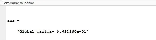
Figure (7) Global maxima
Calculated global maxima is shown in command window and graphical value is founded by taking z coordinate value on clicking highest peak.
Global Maxima analatical value = 0.962960
Global maxima graphical value = 0.9693
Encountered Error:
Encountered Error: This was the error founded and it was on figure output as shown in figure.
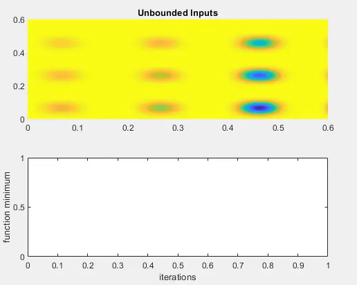
Figure (8) Error
There was error in function program as well as on plotting fopt. All corrections are done by step wise analysis of each lines and corrected format is given in the coding section
Conclusion: Studied and created programs about solving Genetic Algorithm and its different case studies on stalagmite function.
References: