Project 2 - Rankine cycle Simulator
Aim: Develop a program that can solve and display Rankine Cycle parameters by inputs given by the user moreover, to plot T-S and H-S diagrams and to calculate total work done and back work ratio.
Theory and Governing Equations: The Rankine cycle is the basic working cycle of all power plants, in which an operating fluid is constantly evaporated and condensed. The operating fluid chosen is generally influenced by the temperature range available. The idealised Rankine cycle is shown in Figure (1).It is also known as Rankine vapour cycle which converts heat to mechanical energy.
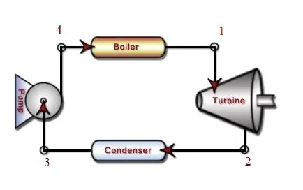
Figure (1) Ideal Rankine Cycle
Figure (2, 3) shows the temperature-entropy (T-S) and enthalpy-entropy (H-S) and diagrams of this cycle. The steps of the Rankine cycle are as follows:
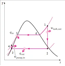
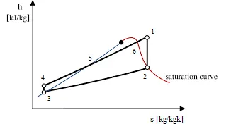
Figure (2) T-S Diagram Figure(3) H-S Diagram
1-2 Isentropic expansion in turbine - In a steam turbine, steam from the boiler expands adiabatically from state 1 to state 2 to produce work before being released to the condenser (partially condensed). The steam interacts with the environment (turbine blades) and loses an amount of enthalpy equal to the amount of work that leaves the system. `wt = h1 – h2` gives the work done by the turbine. The entropy remains unchanged in this stage.
2-3 Isobaric heat rejection in heat exchanger- The cycle is completed in this phase by a constant-pressure mechanism that rejects heat from partially condensed steam. In a cooling circuit, heat is transferred from the vapour to cooling water running via a condenser. As the vapour condenses, the cooling water's temperature rises. `qout = h2 – h1` gives the net heat rejected.
3-4 Isentropic compression in a pump - Centrifugal pumps compress the liquid condensate adiabatically from state 3 to state 4. The liquid condensate is injected into the higher-pressure boiler from the condenser. The fluid's enthalpy and pressure are increased as a result of the surroundings working on it. The entropy, on the other hand, does not alter. `wp = h4 – h3` is the work required for the compressor.
4-1 Isobaric heat addition in boiler – Since the chamber is open to flow in and out, there is a constant-pressure heat transfer to the liquid condensate from an external source during this phase. The feed water is heated to that fluid's boiling point and then evaporated in the boiler. `qi = h4 – h1` is the net heat added. Liquid water is pumped into the boiler and heated to a superheated state.
Net work output: The difference between the turbine work output and the pump work input is the cycle's net work output.
Net work output = `wt - wp`
Back work ratio: It is the ratio of turbine work output to pump work input.
Back work ratio = `(wt)/(wp)`
Coding: The program to solve a Rankine cycle and explanation is given below. Each section is numbered in the program detailed description sections are listed.
clear all
close all
clc

% 1.Headings
fprintf(' %75s',' RANKINE CYCLE SIMULATOR')
fprintf('\n 1-2 Isentropic expansion in Steam turbine')
fprintf('\n 2-3 Constant pressure heat rejection in condenser')
fprintf('\n 3-4 Isentropic compression in the pump')
fprintf('\n 4-1 Constant pressure heat addition in the boiler \n')

% 2.Inputs from the user
T1 = input('\n Enter Temperature at inlet of Turbine T1(Celcius)=')
P1 = input('\n Enter Pressure at inlet of Turbine P1(Bar)=')
P2 = input('\n Enter Pressure at Turbine outlet P2(Bar)=')

% 3.Finding state parameters
% State 1 -Turbine Inlet
h1 = XSteam('h_pT',P1,T1); % Enthalpy at state 1
s1 = XSteam('s_pT',P1,T1); % Entropy at state 1

Tsat_1 = XSteam('Tsat_p',P1); % saturated temp at state 1
sf1 = XSteam('sL_T',Tsat_1);  % saturated liquid entropy at state 1
sg1 = XSteam('sV_T',Tsat_1);  % saturated vapour entropy at state 1
hf1 = XSteam('hV_T',Tsat_1);  % saturated vapour enthalpy at state 1

% State 2 - Condenser inlet
% P2 is .05
s2 = s1; % isentropic expansion
sf2 = XSteam('sL_p',P2);
sg2 = XSteam('sV_p',P2);
hf2 = XSteam('hL_p',P2);
hg2 = XSteam('hV_p',P2);
x2 = ((s2-sf2)/(sg2-sf2));
h2 = hf2+(x2*(hg2-hf2)); % enthalpy at state 2
T2 = XSteam('T_ps',P2,s2); % temperature at state 2
Tsat_2 = XSteam('Tsat_p',P2);

% State 3 - Pump Inlet
P3 = P2; % Constant Pressure
s3 = XSteam('sL_p',P3);    % entropy at state 3
h3 = XSteam('h_ps',P3,s3); % enthalpy at state 3
T3 = XSteam('T_ph',P3,h3); % temperature at state 3

% sg3 = XSteam('sV_p',P3) % saturated vapour entropy

% state 4
P4 = P1; % Constant pressure heat rejection
s4 = s3; % Isentropic expansion
T4 = XSteam('T_ps',P4,s4); % temperature at state 4
h4 = XSteam('h_ps',P4,s4); % enthalpy at state 4
sf4 = XSteam('sL_p',P4);

% points between 4-1
h5 = XSteam('hL_p',P4);    % Enthalpy at state 5
h6 = XSteam('hV_p',P4);    % Enthalpy at state 6
T5 = XSteam('T_ph',P4,h5); % Temp at state 5
T6 = XSteam('T_ph',P4,h6); % Temp at state 6
s5 = XSteam('s_ph',P4,h5);  % Entropy at state 5
s6 = XSteam('s_ph',P4,h6);  % Entropy at state 6


% 3.1.Vapour Dome values
temp = linspace(5,500,500);
for i=1:length(temp)
    s(i)=XSteam('sL_T',temp(i)); % Saturated Liquid Entropy values
    S(i)=XSteam('sV_T',temp(i)); % Saturated Vapour Entropy values
    h(i)=XSteam('hL_T',temp(i)); % Saturated Liquid Enthalpy values
    H(i)=XSteam('hV_T',temp(i)); % Saturated Vapour Enthalpy values
end


% 4.Plotting
% T-S Diagram
figure(1)
line([s1 s2],[T1 T2],'color','g','marker','o','linewidth',2,'markersize',3,'markeredgecolor','k');
hold on
line([s2 s3],[T2 T3],'color','b','marker','o','linewidth',2,'markersize',3,'markeredgecolor','k');
line([s3 s4],[T3 T4],'color','c','marker','o','linewidth',2,'markersize',3,'markeredgecolor','k');
line([s4 s5],[T4 T5],'color','r','marker','o','linewidth',2,'markersize',3,'markeredgecolor','k');
line([s5 s6],[T5 T6],'color','r','marker','o','linewidth',2,'markersize',3,'markeredgecolor','k');
line([s6 s1],[T6 T1],'color','r','marker','o','linewidth',2,'markersize',3,'markeredgecolor','k');
plot(s,temp,'color','k');
plot(S,temp,'color','k');
axis([0 10 0 550]);
xlabel(' Entropy(KJ/Kg)');
ylabel('Temperature (deg-celsius)');
title( 'T-S diagram');
legend('isentropic compression in pump','Heat addition in boiler','isentropic expansion in Steam turbine','Heat rejection in condenser');

% H-S Diagram
figure(2)
line([s1 s2],[h1 h2],'color','g','marker','o','linewidth',2,'markersize',3,'markeredgecolor','k');
hold on
line([s2 s3],[h2 h3],'color','b','marker','o','linewidth',2,'markersize',3,'markeredgecolor','k');
line([s3 s4],[h3 h4],'color','c','marker','o','linewidth',2,'markersize',3,'markeredgecolor','k');
line([s4 s5],[h4 h5],'color','r','marker','o','linewidth',2,'markersize',3,'markeredgecolor','k');
line([s5 s6],[h5 h6],'color','r','marker','o','linewidth',2,'markersize',3,'markeredgecolor','k');
line([s6 s1],[h6 h1],'color','r','marker','o','linewidth',2,'markersize',3,'markeredgecolor','k');
plot(s,h,'color','k');
plot(S,H,'color','k');
axis([0 10 0 5000])
xlabel(' Entropy(KJ/KgK)');
ylabel('Enthalpy (KJ/Kg)');
title( 'H-S diagram');
legend('isentropic compression in pump','Heat addition in boiler','isentropic expansion in Steam turbine','Heat rejection in condenser');

% 5.calculations
wt = h1-h2; % Output work from turbine
wp = h4-h3; % Input work to pump
Net_w = wt-wp; % Net work output
BWR = wp/wt; % Back work Ratio

% 6.Displaying Rankine cycle Parameters
% State 1
fprintf(' At STATE 1');
fprintf('\n  P1= %0.2f Bar',P1);
fprintf('\n  T1= %0.2f Celcius',T1);
fprintf('\n  h1= %0.2f KJ/Kg',h1);
fprintf('\n  s1= %0.2f KJ/KgK \n',s1);
% State 2
fprintf('\n At STATE 2');
fprintf('\n  P2= %0.2f Bar',P2);
fprintf('\n  T2= %0.2f Celcius',T2);
fprintf('\n  h2= %0.2f KJ/Kg',h2);
fprintf('\n  s2= %0.2f KJ/KgK \n',s2);
% State 3
fprintf(' \n At STATE 3');
fprintf('\n  P3= %0.2f Bar',P3);
fprintf('\n  T3= %0.2f Celcius',T3);
fprintf('\n  h3= %0.2f KJ/Kg',h3);
fprintf('\n  s3= %0.2f KJ/KgK \n',s3);
% State 4
fprintf('\n At STATE 4');
fprintf('\n  P4= %0.2f Bar',P4);
fprintf('\n  T4= %0.2f Celcius',T4);
fprintf('\n  h4= %0.2f KJ/Kg',h4);
fprintf('\n  s4= %0.2f KJ/KgK \n',s4);
% Calculations
fprintf('\n  Net work output= %0.4f KJ/Kg \n',Net_w);
fprintf('\n  Back work ratio= %0.4f \n',BWR);
Section (1) – ‘RANKINE CYCLE SIMULATOR’ given as heading using fprintf command and the four processes in the rankine cycle are printed.
Section (2) – The pressure and temperature values of turbine inlet and outlet pressure are to be given by the user.
Section (3) – The four state parameters and points between 4 and 6 are find out using ‘XSteam.m’ function. XSteam can be used multiple ways in order to find any properties of rankine cycle.
Section (3.1) – Vapour dome values are stored in corresponding enthalpy and entropy variables. A for loop is used to find vapour dome values of different temperature values.
Section (4) – This section is drawing T-S and HS diagrams in a separate figures. Line command is used to connect lines between different states and plot command to draw vapour dome curve. Making diagram more vibrant lines are coloured and points are marked with markers. Appropriate units, title and legends are given to the diagram.
Section (5) – This section contains calculations of net work output and back work ratio of rankine cycle by implementing corresponding equations.
Section (6) – Displaying rankine cycle parameters and calculated values using fprintf command.
Outputs: The T-S diagram and H-S diagram obtained shown below.
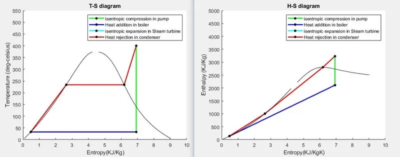
Figure (4) Output Diagrams
The Rankine Cycle state parameters and calculation results obtained in the command window screenshot is given in figure (4).
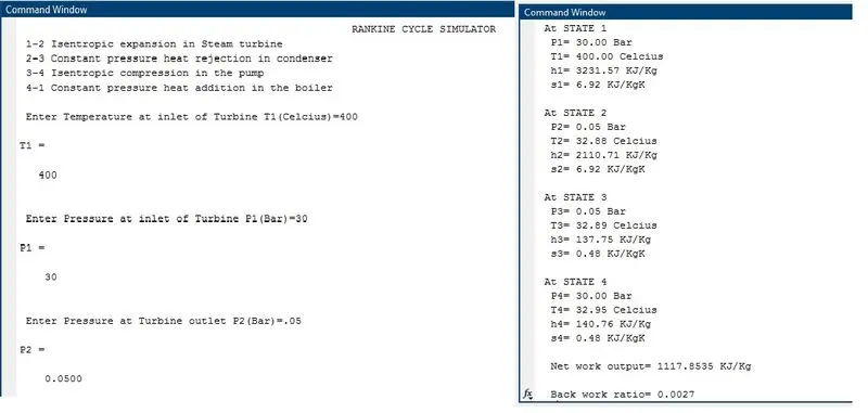
Figure (5) Command window screenshot
Encountered Error:
The obtained diagrams was wrong. The values of statement parameter checked and solved especially state 1 parameters.
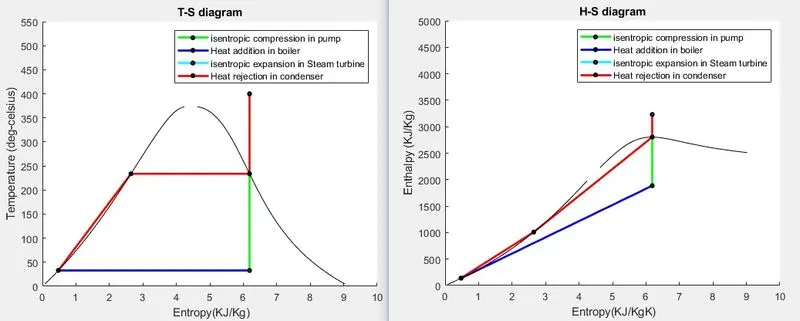
Figure (6) Wrong Diagrams
Conclusions: MATLAB program is created to solve and display a Rankine cycle state parameter and properties by user inputs furthermore, diagrams are plotted and working of cycle is studied.
References: