Week 3 - Solving second order ODEs

Aim: To create matlab program to solve ordinary differential equation that will replicate the motion of a simple pendulum with damping and to animate the movement.

Principle: A mechanical mechanism that oscillates is the simple pendulum. As shown in Figure (1), it is made up of a point mass suspended from a fixed support by a light inextensible string. A gravitational force causes the movement in a vertical plane.

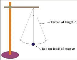
Figure (1) Simple pendulum

Governing Equations:

Equation Of Motion

The Equation of motion of simple pendulum with damping given is (EOM) 

`(d^2theta)/(dt^2 )+b/m*(d theta)/(dt )+g/l*sintheta =0`........(1)`

Where,

g = Gravitational Force in m/s²

m = Mass of the bob in kg

b = Damping Coefficient

L = length of the pendulum in m

Coordinates

As shown in figure (2) the coordinates of simple pendulum points for creating animation is explained below.

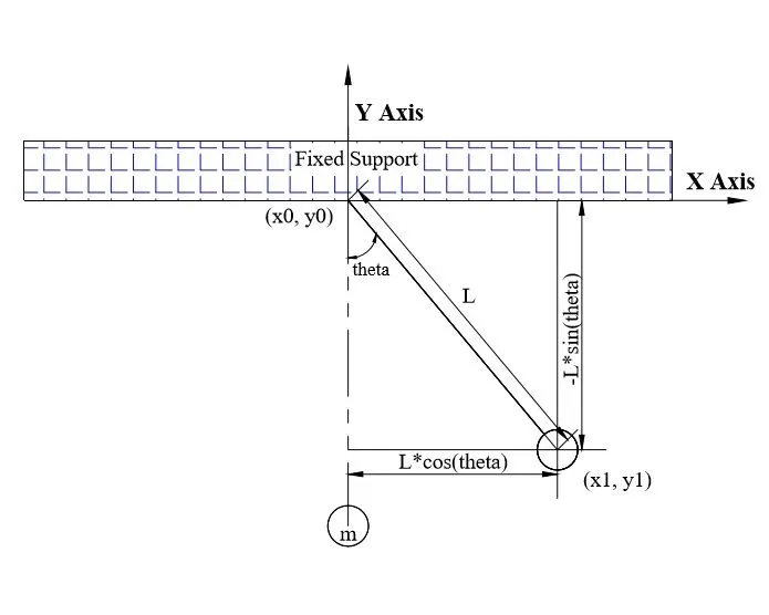
         Figure (2) Coordinate for Animation

Fixed support coordinate = (x0, y0)

End of pendulum coordinate = (x1, y1)

where,

x0 = 0

y0 = 0

x1 = L*sin(theta)

y1 = -L*cos(theta)

Coding:

Function Program

Equation is modified for programming purposes and each step is numbered for explanation.

1. `(d^2theta)/(dt^2 )+b/m*(d theta)/(dt )+g/l*sintheta =0`........(1)`
2. Substituting  `theta = theta1`
3. so `(d theta)/(dt )=(d theta1)/(dt )=theta2`.......(a)`
4. `(d^2theta)/(dt^2 )=(d^2theta1)/(dt^2 )=(d/dt)(d theta1)/(dt )=(d theta2)/(dt)`......(b)`

     Substituting (a) and (b) to equation (1)

    5.`(d theta2)/(dt )=-b/m*theta2-g/l*sintheta1`

     Converting it to matrix form 

    6.`d/dt((theta1),( theta2))=((theta2),(-b/mtheta2-g/lsintheta1))`

    In programming `theta1`= theta1 and `theta2` = theta2

The program code is listed below.

function[dtheta_dt] = ode_func(t,theta,b,g,L,m)
theta1 = theta(1)
theta2 = theta(2)
dtheta1_dt = theta(2);
dtheta2_dt = -(b/m)*theta2-(g/L)*sin(theta1); % Equation of motion
dtheta_dt = [dtheta1_dt; dtheta2_dt] % Matrix format
end

function[dtheta_dt] = ode_func(t,theta,b,g,L,m) - Creating a Function with output variable  dtheta_dt and input variables t, theta, b, g, L, and m. Function name here is ode_func.

theta1 = theta(1)- To store theta(1) values in theta1 variable .

theta2 = theta(2) )- To store theta(2) values in theta2 variable .

dtheta1_dt = theta(2); - dtheta1_dt variable assigned to store theta(2) values(step3).

dtheta2_dt = -(b/m)*theta2-(g/l)*sin(theta1); - Step 5 equation is applied.

dtheta_dt = [dtheta1_dt; dtheta2_dt] – Values are Stored in a column matrix where first column dtheta1_dt value and dtheta2_dt values in second column (step 6).

end –End of function.

Main Program

The program for solving Ordinary Differential Equation of Simple Pendulum with damping and to animate the movement is shown. Explanation of program is divided into several parts for better understanding.

clear all
close all
clc

% Inputs (given data)
b = 0.05; % Damping Coefficient
g = 9.81; % Gravitational Force
L = 1;    % Length of pendulum
m = 1;    % Mass of bob

% Initial Conditions
theta_0 = [0;3];  % Angular Displacement = 0 & Angular Velocity = 3

% Time Points
t_span = linspace(0,20,300); % Time is 20 seconds and divided to 300 portions

% Solve ODE 
[t, solutions] = ode45(@(t, theta) ode_func(t, theta, b , g, L, m), t_span, theta_0)

% Plot
figure(1)                 % To open new window
plot(t, solutions(:,1))   % To plot Angular Displacement w.r.t time
hold on                   % To hold above lines 
plot(t, solutions(:,2) )  % To plot Angular Velocity w.r.t time
xlabel('Time in sec')     % To show Time in sec in X axis 
ylabel('Rad and Rad/sec') % To show Rad and Rad/sec in Yaxis 
legend('Angular Displacement','Angular Velocity') % To Identify both lines
title('Motion of Simple Pendulum')                % To give Motion of Simple Pendulum as title

% Animation
ct = 1;    % counting variable

for i=1:length(solutions(:,1)) 
    angles = solutions(i,1); 
    
    % Coordinates of Fixed Support
    x0 = 0;
    y0 = 0;
    
    % Coordinates of Pendulum end
    x1 = L*sin(angles);
    y1 = -L*cos(angles);
    
    %Plotting
    figure(2)
    
    % To plot Fixed support line
    plot([-0.4 0.4],[0 0],'color','c','linewidth',6)
    hold on
    
    % The string line connecting support and bob
    plot([x0 x1], [y0 y1],'color','b','linewidth',2) 
    
    % To plot Mass or bob
    plot(x1, y1, 'o','markerfacecolor','k','markersize',15) 
    axis([-1.5 1.5 -1.5 0.5]) % Graph Dimenisions
    
    % Heading
    text(-0.57,0.25,'Motion of Simple Pendulum')
    text(-0.15,0.15,num2str(t(i)))
    pause(0.001)
    hold off
    
    M(ct)=getframe(gcf);
    ct = ct+1;
end
% Movie Generation
movie(M)
videofile=VideoWriter('Simple_Pendulum.avi');
open(videofile)
writeVideo(videofile, M)
close(videofile)

• ode45

The Function ode45 function needs to be explained. It is a function used for ordinary differential equations solving. A typical use of ode45 is given below.

Syntax: [tsolutions, ysolutions] = ode45 (@(t,y) fname(t, y), [t0, tend], y0);

tsolutions, ysolutions – Solution vectors, matlab returns ysolutions for each time tsolutions.

fname – Function that returns dy = f(t,y)

t0, y0 – Initial conditions representing y(t0) = y0

tend – Final value until which solution is desired.  

The usage in program: [t, results] = [t, solutions] = ode45 (@(t, theta) ode_func(t, theta, b , g, L, m), t_span,theta_0)

[t, results] – Solution vectors, matlab returns results for each time t.

(t, theta) – Declaring that it is a function of t and theta that is dependant and independent variables.

ode_func(t, theta, b, g, L, m) – ode_func Function calling with t, theta, b, g, L and m as input variables.

t_span – Time array to set initial condition.

theta_0 – Initial condition.

• Animation

To animate motion of Pendulum for loop is used and it’s logic and each line is explained below.

ct = 1; - Counting variable ct.

for i=1:length(solutions(:,1))- Start of for loop, counting variable is i, loop runs till last digit of solutions matrix first column. The values of displacement are in first column.

    angles = solutions(i,1); - It is to access all elements in the displacement array. This is to locating coordinates for plot all points during motion.

    x0 = 0; ­- x coordinate of fixed support.

    y0 = 0; - y coordinate of fixed support.

    x1 = L*sin(angles); - x coordinate of Pendulum end.

    y1 = -L*cos(angles); - y coordinate of Pendulum end.

    figure(2) – To open a new window.

    plot([-0.4 0.4],[0 0],'color','c','linewidth',6) - To draw support line.

    hold on  - To hold the previous line with the current one.

    plot([x0 x1], [y0 y1],'color','b','linewidth',2) - To plot string attached between support and bob.

    plot(x1, y1, 'o','markerfacecolor','k','markersize',15) - To mark bob at the end of string.

    axis([-1.5 1.5 -1.5 0.5]) – Setting  graph dimensions.

    text(-0.57,0.25,'Motion of Simple Pendulum') – To give a heading as ‘Motion of Simple Pendulum’ in the plot by giving X and Y coordinate values.

    text(-0.15,0.15,num2str(t(i))) - To show time in seconds.

    pause(0.001) - pauses execution for 0.001 seconds for suitable speed representation of pendulum movements and to reduce video len.

    hold off – Clear all axis properties and plots.

    M(ct)=getframe(gcf); - In a for loop, getframe is frequently used to record many frames into a m(ct) array. ct values in incremented in each iteration and corresponding frame is captured.

    ct = ct+1; ; - Incremented by one in each for loop iteration.

end- End of for loop.

movie(M)- plays the movie.

videofile=VideoWriter('Simple_Pendulum.avi'); - Defines a VideoWriter object to write video data to an AVI file with name Simple_pendulum.

open(videofile) - open command is for opening  file for writing video data.

writeVideo(videofile, m) - writeVideo command is  for writing video data to file.

close(videofile) - close command is for closing  file after writing video data.

Encountered Errors: There are some encountered errors during development on program and some of them are listed below.

• Error in the syntax of ode45 function.

                      Figure(3) Error in ode45 syntax

Missed to mention initial conditions additionally, mismatch in the parentheses usages.

Wrong Lines: [t, solutions] = ode45(@(t, theta) ode_func(t, theta, b , g, L, m)

Corrected Lines: [t, solutions] = ode45(@(t, theta) ode_func(t, theta, b , g, L, m), t_span, theta_0)

• The Animation was getting wrong because of coding errors found out those mistakes and corrected for expected output.

            

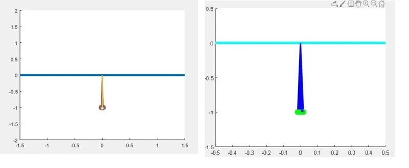
                                Figure (4) Wrong Animations

This was the first time animation outputs and identified those errors.The basic problem was wrong usage of hold on functions and order of plot lines. Identified those errors and the corrected codes are listed above in the main program.

• Everything was perfect except the amplitude of pendulum motion, line by line inspections and manual calculations spotted the mistakes and rectified those lines.

Wrong Lines:         x1 = L*sind(angles); 

                            y1 = -L*cosd(angles);

Corrected Lines:      x1 = L*sin(angles);

                            y1 = -L*cos(angles);  

The angles was in radians not in degrees.

Outputs: The graph of Angular Displacement and Angular Velocity with respect to time is shown in the below figure.

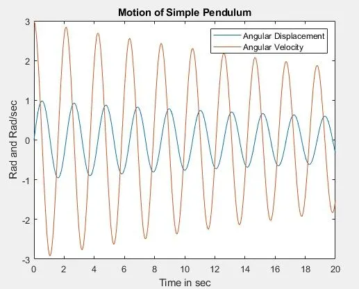
                       Figure (5) Graph

Animation Link:https://youtu.be/AfAG0nJA-7g

Conclusions: Solved second order differential equation of simple pendulum with damping using matlab and created animation video of its motion.