Week 4.1 - Genetic Algorithm
MATLAB CODE TO OPTIMISE THE STALAGMITE FUNCTION USING GENETIC ALGORITHM AND TO FIND GLOBAL MAXIMA OF FUNCTION
Genetic Algorithm (GA) :
A genetic algorithm is a search heuristic that is inspired by Charles Darwin’s theory of natural evolution. This algorithm reflects the process of natural selection where the fittest individuals are selected for reproduction in order to produce offspring of the next generation.
Notion of GA:
The process of natural selection starts with the selection of fittest individuals from a population. They produce offspring which inherit the characteristics of the parents and will be added to the next generation. If parents have better fitness, their offspring will be better than parents and have a better chance at surviving. This process keeps on iterating and at the end, a generation with the fittest individuals will be found.
This notion can be applied for a search problem. We consider a set of solutions for a problem and select the set of best ones out of them.
Five phases are considered in a genetic algorithm.
- Initial population
- Fitness function
- Selection
- Crossover
- Mutation
1. Initial Population:
The process begins with a set of individuals which is called a Population. Each individual is a solution to the problem you want to solve.
An individual is characterized by a set of parameters (variables) known as Genes. Genes are joined into a string to form a Chromosome (solution).
In a genetic algorithm, the set of genes of an individual is represented using a string, in terms of an alphabet. Usually, binary values are used (string of 1s and 0s). We say that we encode the genes in a chromosome.
2. Fitness function:
The fitness function determines how fit an individual is (the ability of an individual to compete with other individuals). It gives a fitness score to each individual. The probability that an individual will be selected for reproduction is based on its fitness score.
3. Selection:
The idea of selection phase is to select the fittest individuals and let them pass their genes to the next generation.
Two pairs of individuals (parents) are selected based on their fitness scores. Individuals with high fitness have more chance to be selected for reproduction.
4. Crossover:
Crossover is the most significant phase in a genetic algorithm. For each pair of parents to be mated, a crossover point is chosen at random from within the genes.
Offspring are created by exchanging the genes of parents among themselves until the crossover point is reached.
The new offspring are added to the population.
5. Mutation:
In certain new offspring formed, some of their genes can be subjected to a mutation with a low random probability. This implies that some of the bits in the bit string can be flipped.Mutation occurs to maintain diversity within the population and prevent premature convergence.
6. Termination:
The algorithm terminates if the population has converged (does not produce offspring which are significantly different from the previous generation). Then it is said that the genetic algorithm has provided a set of solutions to our problem.
Stopping Criteria for GA:
-
Generations — The algorithm stops when the number of generations reaches the value of Generations.
-
Time limit — The algorithm stops after running for an amount of time in seconds equal to Time limit.
-
Fitness limit — The algorithm stops when the value of the fitness function for the best point in the current population is less than or equal to Fitness limit.
Syntax for 'ga' in MATLAB:
[Inputs, Fvals] = ga(fun,nvars,A,B,Aeq,Beq,lb,ub,nonlcon,Intcon,options)
fun : The function which is to be optimised.
nvars : The dimension (number of design variables) of fun.
A,B : Finds a local minimum x to fun, subject to the linear inequalities A*x<=B. ga evaluates the matrix product A*x as if x is transposed.
Aeq,Beq : Finds a local minimum x to fun, subject to the linear equalities Aeq*x=beq and A*x<=B. ga evaluates the matrix product Aeq as if x is transposed.
lb,ub : defines a set of lower and upper bounds on the design variables, x, so that a solution is found in the range lb<=x<=ub.
nonlcon,Intcon,options : minimizes with the default optimization parameters replaced by values in options. Create options using optimoptions.
[Note : Use [ ] if linear and non linear inequalities or equalties do not exist.]
Stalagmite function:
Stalagmite function code:
% Stalagamite function
function f=stalagmite(input)
x=input(1);
y=input(2);
pie=22/7;
f1_x =(sin(5.1*pie*x+0.5))^6;
f1_y =(sin(5.1*pie*y+0.5))^6;
f2_x =exp(-4*log(2)*((x-0.0667)^2)/0.64);
f2_y =exp(-4*log(2)*((y-0.0667)^2)/0.64);
f=-(f1_x*f1_y*f2_x*f2_y);
end
Code Explanation:
- Line-2:----> Creating a function with name stalagmite and inputs as input and f ans output of function.
- Line-3:----> Storing the first row of input values in x.
- Line-4:----> Storing the second row of input values in y.
- Line-4:----> defining pie as 22/7.
- Line-5 to 10:----> Creating lines of codes using stalagmite function formulae and ending the function and returning the the value of f to function.
Note : The -ve sign for value of f is used because to find global maxima in ga optimisation since ga only gives global minima of a function.
Code to optimise stalagmite function:
% MATLAB code to optimise the stalagmite function and find the global maxima of the function.
clear all
close all
clc

% Inputs
x=linspace(0,0.9,150);
y=linspace(0,0.9,150);

% Meshgrid
[xx,yy] = meshgrid(x,y);

for i=1:length(xx)
    for j=1:length(yy)
        input(1) =xx(i,j);
        input(2) =yy(i,j);
        f(i,j)=stalagmite(input);
    end
end

% Plotting
figure(1)
surfc(xx,yy,-f)
view(45,20)
title('Stalagmite')
shading interp
xlabel('x')
ylabel('y')
zlabel('Function Value')

num_cases=50;

% Statistical behaviour of GA (Genetic Algorithm)

tic
for i=1:num_cases
    [inputs1,f_1]=ga(@stalagmite,2);
    x1(i)=inputs1(1);
    y1(i)=inputs1(2);
    f1(i)=f_1;
end
study_time_1=toc;     % Time taken to evalate the code from tic

% Plotting
figure(2)
subplot(2,1,1)   % First plot in figure(2)
hold on
surfc(xx,yy,-f)
view(45,20)
title('Statistical behaviour of Genetic Algorithm (GA)')
shading interp
plot3(x1,y1,-f1,'marker','o',MarkerFaceColor='r')
xlabel('x')
ylabel('y')
zlabel('Function Value')

subplot(2,1,2)    % second plot in figure(2)
plot(-f1)
xlabel('Iteration')
ylabel('Function Value')


% Statistical behaviour of GA with bounds

tic
for i=1:num_cases
    [inputs2,f_2]=ga(@stalagmite,2,[],[],[],[],[0 0],[0.6 0.6]);
    x2(i)=inputs2(1);
    y2(i)=inputs2(2);
    f2(i)=f_2;
end
study_time_2=toc;    % Time take to evaluate code from tic

% Plotting
figure(3)
subplot(2,1,1)    % First plot in figure(3)
hold on
surfc(xx,yy,-f)
view(45,20)
title('Statistical behaviour of GA with bounds')
shading interp
plot3(x2,y2,-f2,'marker','o',MarkerFaceColor='r')
xlabel('x')
ylabel('y')
zlabel('Function Value')

subplot(2,1,2)    % Second plot in figure(3)
plot(-f2)
xlabel('Iteration')
ylabel('Function Value')


% Statistical behaviour of GA with bounds and increasing Population Size
options=optimoptions('ga','PopulationSize',500);
tic
for i=1:num_cases
    [inputs3,f_3]=ga(@stalagmite,2,[],[],[],[],[0;0],[1;1],[],[],options);
    x3(i)=inputs3(1);
    y3(i)=inputs3(2);
    f3(i)=f_3;
end
study_time_3=toc;    % Time taken to evalute the code from tic

% Plotting
figure(4)
subplot(2,1,1)    % First plot in figure(4)
hold on
surfc(xx,yy,-f)
view(45,20)
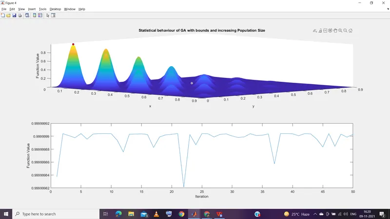
title('Statistical behaviour of GA with bounds and increasing Population Size')
shading interp
plot3(x3,y3,-f3,'marker','o',MarkerFaceColor='r')
xlabel('x')
ylabel('y')
zlabel('Function Value')

subplot(2,1,2)    % Second plot in figure(4)
plot(-f3)
xlabel('Iteration')
ylabel('Function Value')

% Printig the values of study time for each case
fprintf('Study time-1 = %d \n',study_time_1)
fprintf('Study time-2 = %d \n',study_time_2)
fprintf('Study time-3 = %d \n',study_time_3)

% Printing coordinates of global maxima of function
fprintf('The x and y values at global maxima of the stalagmite function = (%d, %d) \n',inputs3(1),inputs3(2))
fprintf('The maximum value of function is %d \n',-f_3)
Code Explanation:
- Line-2: close all ----> closes all the Plots.
- Line-3: clear all ----> clears all the variables in the workspace.
- Line-4: clc ----> clears the command window.
- Line-7 and 8:----> Creates a input values of x and y using linspace command.
- Line-11:----> Meshgrid of x and y and storing the values in xx and yy.
- Line-13 to 19:----> using multiple for loops to to give input values to stalagmite function and store the function values in f.
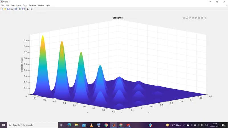
- Line-22 to 29:----> in figure 1 creating a surface plot of xx,yy and -f (Since the function values are stored -ve for global maxima calculation), with view of azimuth angle 45 degrees and elevation angle of 20 degrees. The title of figure being stalagmite with x,y,x labels of x,y, function value respectively. The use of shading interp is made to remove grid lines in plot.
- Line-31:----> storing 50 in variable num_cases.
- Use of multiple iterations is made because for each time of optimisation ga returns different values and to make ga otimise accurately the following cases are done.
- Case-1: (Statistical behaviour of GA)
- Line-35:----> tic command to start the run time of code.
- Line-36 to 41:----> using for loop the gd is made to optimise stalagmite function 50 times and store the optimisation results in x1,y1 and function values in f1 in each iteration of for loop.
- Line-42:----> Storing the run time of for loop from tic to tac in study_time_1 Variable.
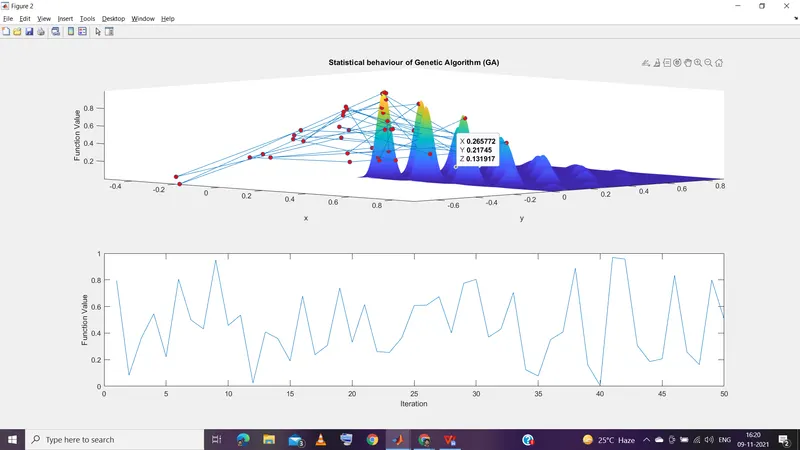
- Line-46:----> dividing figure 2 into 2 by 1 gird and ploting the below plots inside 1st row of grid.
- Line-48 to 52:----> Plotting a surface plot of xx,yy and -f and a 3d plot with points x1,y1 and-f1(The function returns negative values for global maxima) with marker o and face colour red. the ttle for the pot is given using title command and x,y,z labels are given.
- Line-57 to 60:----> In the second row of figure 2 a plot of function values is made with x and y labels as aiteration and Function values respectively.
- Case-2: (Statistical behaviour of GA with bounds)
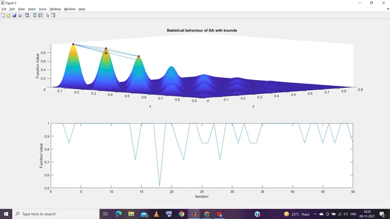
- Line-64 to 91:----> The code from lines 33 to 60 is being repeated with new variables and main difference is setting lower and upper bounds in ga command. This change makes the ga command to search for optimium values inside the limits.
- Case-3: (Statistical behaviour of GA with bounds and increasing Population Size)
- Line-96:----> Using optimoptions command the population size in ga command is changed from default value to 500.
- Line-97 to 122:----> Code of lines from 64 to 91 is repetated with new variables to store values. Since the population size is changed to 500 the ga command will optimise the stalagmite function according to the changes and gives optimum and accurate solution.
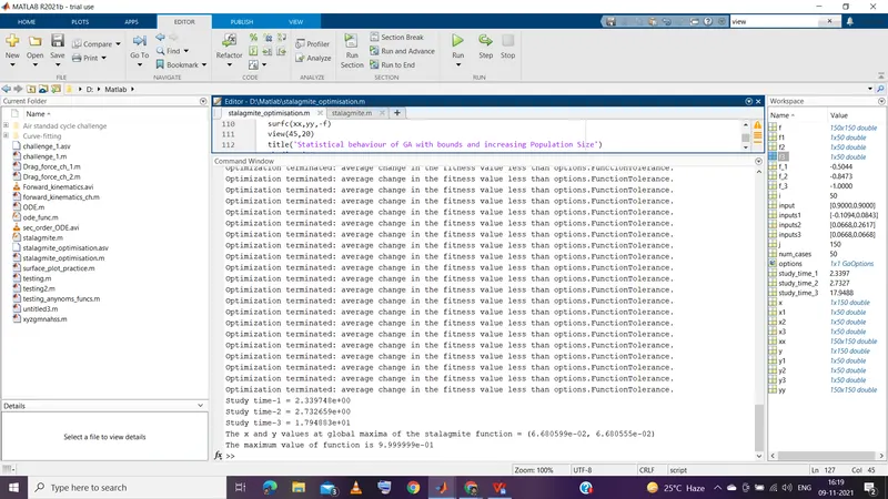
- Line-125 to 127:----> Printing the study time values for each case in command window.
- Line-130 and 131:----> Printing the coordinates of global maxima and the maximum value of stalagmite function.
Command window Output:
Output Plots:
Errors Faced:
1. Small errors for coding like no proper usuage of variables in commands, use of paranthesis etc....
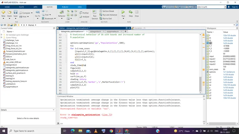
2. Error in usuage of tic and toc commands.
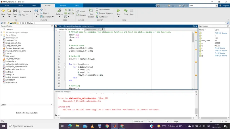
3. The stalagmite function should have a single input matrix parameter since ga doest not allow multiple input functions.
References: