CURVE FITTING
CURVE FITTING
Contents:
1. What is Curve fitting?
2. MATLAB Code to fit a linear and cubic polynomial for the Cp data.
3. MATLAB Code to show splitwise method.
4. Parameters used to measure the fitness characteristics for both the curves.
5. Q&A
6. References
1. What is Curve fitting?
Curve fitting is the process of constructing a curve, or mathematical functions, which possess the closest proximity to the real series of data. By curve fitting, we can mathematically construct the functional relationship between the observed dataset and parameter values, etc. It is highly effective in the mathematical modeling of some natural processes.
2. MATLAB Code to fit a linear and cubic polynomial for the Cp data.
% Code to fit linear and cubic polynomial for Cp data
clear all
close all
clc

% Loading the values from data
cp_data=load('data');
temperatures=cp_data(:,1);
cp=cp_data(:,2);

% Creating a linear polynomial
linear_coeffs=polyfit(temperatures,cp,1);
linear_predicted_cp=polyval(linear_coeffs,temperatures);

% Calculating SSR and SSE Matrices for linear fit
mean_linear=mean(linear_predicted_cp);    % Mean of linear fit values

for i=1:length(linear_predicted_cp)
ssr_linear(i,1) = (linear_predicted_cp(i)-mean_linear)^2;
sse_linear(i,1)= (cp(i)-linear_predicted_cp(i))^2;
end

% Summation
SSR_linear=sum(ssr_linear);
SSE_linear=sum(sse_linear);

% Calculating R_square and Root mean squared error (RMSE)
R_square_linear=SSR_linear/(SSR_linear+SSE_linear);
RMSE_linear=(SSE_linear/length(linear_predicted_cp))^0.5;

% Printing SSE, R_square and RMSE
fprintf('SSE_linear= %dn',SSE_linear)
fprintf('R_Square_linear= %dn',R_square_linear)
fprintf('RMSE_linear = %dnn',RMSE_linear)


% Creating cubic polynomial
cubic_coeffs=polyfit(temperatures,cp,3);
cubic_predicted_cp=polyval(cubic_coeffs,temperatures);

% Calculating SSR and SSE Matrices for cubic polynomial
mean_cubic=mean(cubic_predicted_cp);      % Mean of cubic fit values

for i=1:length(cubic_predicted_cp)
ssr_cubic(i,1) = (cubic_predicted_cp(i)-mean_cubic)^2;
sse_cubic(i,1)= (cp(i)-cubic_predicted_cp(i))^2;
end

% Summation
SSR_cubic=sum(ssr_cubic);
SSE_cubic=sum(sse_cubic);

% Calculating R_square and Root mean squared error (RMSE)
R_square_cubic=SSR_cubic/(SSR_cubic+SSE_cubic);
RMSE_cubic=(SSE_cubic/length(cubic_predicted_cp))^0.5;

% Printing SSE, R_square and RMSE
fprintf('SSE_cubic = %dn',SSE_cubic)
fprintf('R_Square_cubic = %dn',R_square_cubic)
fprintf('RMSE_cubic = %dn',RMSE_cubic)

% Plotting
plot(temperatures,cp,'color','k','LineWidth',2)
hold on
plot(temperatures,linear_predicted_cp,'color','r','LineWidth',2)
plot(temperatures,cubic_predicted_cp,'color','c','LineWidth',2)
title('Linear Polynomial and Cubic Polynomial fits')
grid on
axis([200 3700 800 1600])
xlabel('Temperature-(Kelvin)')
ylabel('Specific heat (C_p)-KJ/Kmole-K')
legend('Actual Curve','Linear polynomial curve fit','Cubic Polynomial curve fit')
Code Explaination:
- Line-2: close all ----> closes all the Plots.
- Line-3: clear all ----> clears all the variables in the workspace.
- Line-4: clc ----> clears the command window.
- Line-6 to 9: ----> Loading the values of data in variables temperatures and cp using load command.
- Line-12: ----> Evaluating the values of constants in the linear equation using polyfit command and storing the values of constants in variable linear_coeffs using the values from data.
- Line-13: ----> Solving the linear polynomial using linear_coeffs and temperature values from data and storing the solutions of linear polynomial created in the variable linear_predicted_cp.
- Line-16: ----> Using mean command calculating the mean of values in linear_predicted_cp.
- Line-18 to 21: ----> In for loop which is iterated from 1 to length of linear_predicted_cp the matrices for values of ssr and and sse are calculated using formulae ssr=(linear_predicted_cp-mean)^2 sse=(Cp values from data - predicted Cp values using fit)^2 for each iteration of for loop.
- Line-24 to 25: ----> Summation of the values of ssr and sse.
- Line-27 to 29: ----> Calculating R_square and Root mean squared error using formulae R_square_linear = SSR_linear/(SSR_linear+SSE_linear) RMSE_linear = (SSE_linear/length(linear_predicted_cp))^0.5
- Line-31 to 34: ----> The values of SSE,R_square and RMSE are printed in command window using fprintf command.
- Line-37 to 60: ----> The lines 12 to 34 explain the cretion of linear fit ,the same is repeated from lines 37 to 60 for creating the cubic poynomial fit using different variables to store data and in polyfit command using degree of polynomial to be 3.
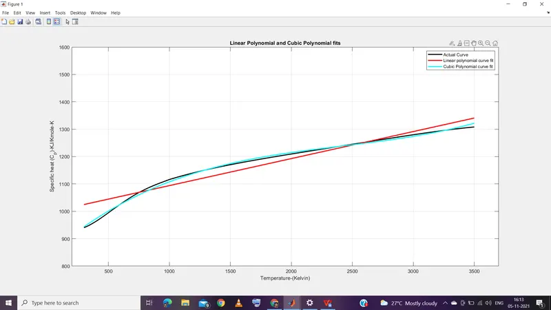
- Line-63 to 66: ----> Creating plots for temperature vs Cp from data, temperature Vs linear predicted Cp and temperature Vs Cubic poynomial fit in a single figure using hold on command.
- Line-67 : ----> Giving title to plot using title command.
- Line-68: ----> Enable the Grid on plot.
- Line-69: ----> Setting the limits of Axis taken as, X-AXIS = 200 TO 3700
Y-AXIS = 800 TO 1600
- Line-70: ---> Labels X-axis of plot naming as Temperature-(Kelvin).
- Line-71: ---> Labels Y-axis of plot naming as Specific heat (C_p)-KJ/Kmole-K.
- Line-72: ---> Information about the curves in single plot in top-right corner of the plot.
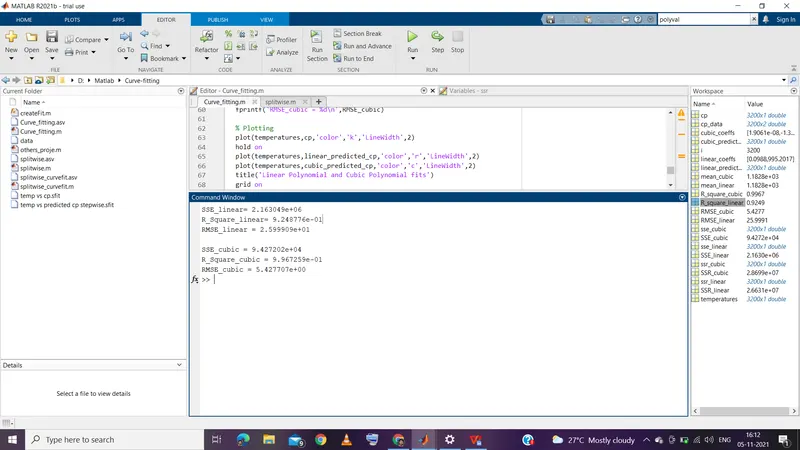
Command window output:
Output plot:
3. MATLAB Code to show splitwise method.
%Splitwise method
clear all
close all
clc

% Loading the values from data
cp_data=load('data');
temperatures=(cp_data(:,1));
cp=cp_data(:,2);

% Inputs
step_size=100;
stepwise_predicted_cp=[];

% Stepwise splitting and Calculation
for i=1:step_size:length(temperatures)
    j=i+step_size-1;
    linear_coeffs=polyfit(temperatures(i:j),cp(i:j),1);
    predicted_cp=polyval(linear_coeffs,temperatures(i:j));
    stepwise_predicted_cp = [stepwise_predicted_cp;predicted_cp];
end

% Calculating SSR and SSE Matrices.
mean=mean(stepwise_predicted_cp);    % Mean of stepwise fit values

for i=1:length(stepwise_predicted_cp)
ssr(i,1) = (stepwise_predicted_cp(i)-mean)^2;
sse(i,1)= (cp(i)-stepwise_predicted_cp(i))^2;
end

% Summation
SSR=sum(ssr);
SSE=sum(sse);

% Calculating R_square and Root mean squared error (RMSE) for fit.
R_square=SSR/(SSR+SSE);
RMSE=(SSE/length(stepwise_predicted_cp))^0.5;

% Printing SSE, R_square and RMSE
fprintf('SSE=%dn',SSE)
fprintf('R_Square_Splitwise = %dn',R_square)
fprintf('RMSE_splitwise = %d n',RMSE)

% Plotting
plot(temperatures,stepwise_predicted_cp,'color','c','LineWidth',6)
hold on
plot(temperatures,cp,'color','r','LineWidth',2)
title('Split-wise Fit')
legend('Stepwise Curve','Actual curve')
grid on
axis([200 3700 800 1600])
xlabel('Temperature-(Kelvin)')
ylabel('Specific heat (C_p)-KJ/Kmole-K')
Code Explaination:
- Line-2: close all ----> closes all the Plots.
- Line-3: clear all ----> clears all the variables in the workspace.
- Line-4: clc ----> clears the command window.
- Line-6 to 9: ----> Loading the values of data in variables temperatures and cp using load command.
- Line-12 and 13: ----> giving stepsize as 100 and creating a empty matrix of name stepwise_predicted_cp
- Line-16 to 20: ----> In for loop running from 1 to length of temperature values with a step size of 100. In the for loop creating sets of limits using formulae j=i+step_size-1 thus creating a set of range in each iteration of for loop. fitting a linear polynomial curve fit using the divided set of range values. Storing the values of fit in matrix colum for each iteration and ending the for loop.
- Line-24: ----> Using mean command calculating the mean of values in linear_predicted_cp.
- Line-26 to 29: ----> In for loop which is iterated from 1 to length of linear_predicted_cp the matrices for values of ssr and and sse are calculated using formulae ssr=(linear_predicted_cp-mean)^2 sse=(Cp values from data - predicted Cp values using fit)^2 for each iteration of for loop.
- Line-32 to 33: ----> Summation of the values of ssr and sse.
- Line-36 to 37: ----> Calculating R_square and Root mean squared error using formulae R_square_linear = SSR_linear/(SSR_linear+SSE_linear) RMSE_linear = (SSE_linear/length(linear_predicted_cp))^0.5
- Line-39 to 42: ----> The values of SSE,R_square and RMSE are printed in command window using fprintf command.
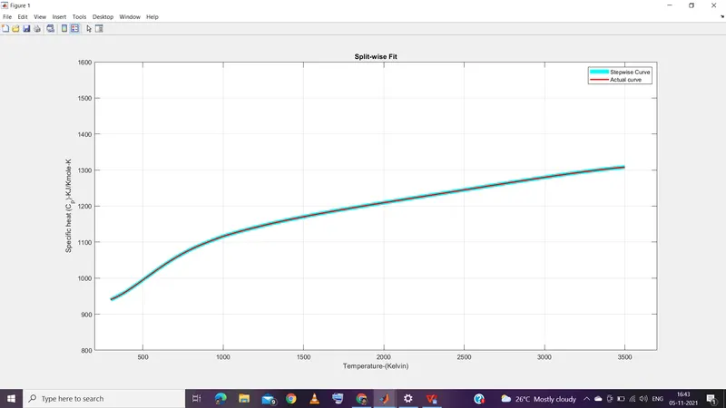
- Line-45 to 47: ----> Creating plots for temperature vs Cp from data, temperature Vs stepwise_predicted_cp in a single figure using hold on command.
- Line-48 : ----> Giving title to plot using title command.
- Line-49: ---> Information about the curves in single plot in top-right corner of the plot.
- Line-50: ----> Enable the Grid on plot.
- Line-51: ----> Setting the limits of Axis taken as, X-AXIS = 200 TO 3700
Y-AXIS = 800 TO 1600
- Line-52: ---> Labels X-axis of plot naming as Temperature-(Kelvin).
- Line-53: ---> Labels Y-axis of plot naming as Specific heat (C_p)-KJ/Kmole-K.
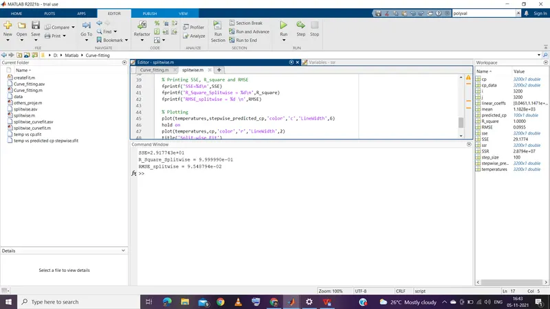
Command window output:
Output plot:
4. Parameters used to measure the fitness characteristics for both the curves.
- The sum of squared errors (SSE)
- R-square
- Root mean squared error (RMSE)
SSE:
SSE is the sum of the squared differences between each observation and its group's mean. It can be used as a measure of variation within a cluster. If all cases within a cluster are identical the SSE would then be equal to 0.
The formula for SSE is:
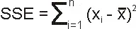
where x¯">¯xx¯ is the mean of all values of x.
For best fit the value of SSE should be small when compared to other fits.
In above linear,cubic and splitwise fits the values of SSE are 2.163049089179785e+06, 9.427202052073379e+04 and 29.177428869648450 respectively. From the values we can observe that best fit is
Splitwise fit > Cubic polynomial fit > Linear polynomial fit
R-square:
R-squared (R2) is a statistical measure that represents the proportion of the variance for a dependent variable that's explained by an independent variable or variables in a regression model. Whereas correlation explains the strength of the relationship between an independent and dependent variable, R-squared explains to what extent the variance of one variable explains the variance of the second variable.
The formula for R-square is:
R_square = SSR / (SSR+SSE).
Where,
SSR=1-(Unexplained variance/total variance)
R-squared values range from 0 to 1 and are commonly stated as percentages from 0% to 100%. An R-squared of 100% means that all movements of a security (or another dependent variable) are completely explained by movements in the index (or the independent variable(s) you are interested in).
In above linear,cubic and splitwise fits the values of R^2 are 9.248776e-01, 9.967259e-01 and 9.999990e-01 respectively. From the values we can observe that best fit is
Splitwise fit > Cubic polynomial fit > Linear polynomial fit
Root Mean Square Error (RMSE):
It is the Standard deviation of the residuals (prediction errors). Residuals are a measure of how far from the regression line data points are; RMSE is a measure of how spread out these residuals are. In other words, it tells you how concentrated the data is around the line of best fit. Lesser the value of RMSE greater the fit.
RMSE=(SSEN)12">(SSEN)12(SSEN)12
In above linear,cubic and splitwise fits the values of RMSE are 2.599909e+01, 5.427707e+00 and 9.548794e-02 respectively. From the values we can observe that best fit is
Splitwise fit > Cubic polynomial fit > Linear polynomial fit
5. Q&A:
- How to make a curve fit perfectly?
To make a curve fit perfectly we can use splitwise method as discussed in the above code. Splitwise method splits the data to be fitted creates fits for each set of data thus giving us perfect fit. more the number of divisions greater the fit. We can also increase the fitness by increasing the order of the polynimal used for fitting.
- How to get the best fit?
To get best fit we can comapre the values of SSE, R^2 and RMSE. To get best fit values of SSE and RMSE should be small when compared to other fits. R^2 values range from 0 to 1 and for a best fit the value of R^2 should be greater than 0.95.
- What could be done to improve the cubic fit?
we can use center and scale to improve the cubic fit or we can use splitwise method to improve cubic fit as the method does not need to increase the degree to get best fit
6. References