Solving second order ODEs

Solving Second Order ODEs

Ordinary differential equation taken:

In the above equation,

g = gravity in m/s2,

L = length of the pendulum in m,

m = mass of the ball in kg,

b=damping coefficient.

Problem taken:

Write a program in Matlab that will simulate the pendulum motion. Use

L=1 metre,

m=1 kg,

b=0.05.

g=9.81 m/s2.

Simulate the motion between 0-20 sec, for angular displacement=0,angular velocity=3 rad/sec at time t=0.

Matlab Code:

% Matlab code to simulate pendulum motion
clear all
close all
clc

% inputs
b=0.05;  % damping coefficient
g=9.81;  % gravity in m/s2,
l=1;     % length of the pendulum in m,
m=1;     % mass of the ball in kg,

% initial conditions
theta_0=[0;3];

% time points
t_span=linspace(0,20,300);

% Solve ODE using ode45
[t,results]=ode45(@(t,theta) ode_func(t,theta,b,g,l,m),t_span,theta_0);

% Plotting Angular displacement and Angular velocity.
hold on
plot(t,results(:,1),'Color','r') % plot for Angular displacement
plot(t,results(:,2),'Color','b') % plot for Angular velocity
xlabel('Time')
ylabel('Plot') 
legend('Angular displacement','Angular velocity')


ct=1;
for i=1:length(t)

    % Coordinates of pendulum with respect to angular displacement
    x0=0;
    y0=0;
    x1=l*sin(results(i,1))
    y1=-l*cos(results(i,1)) 
    
    % Plotting the pendulum movement.
    figure(2)
    plot([x0,x1],[y0,y1])
    hold on
    plot([-1.5 1.5],[0 0],'color','r','LineWidth',3)
    axis([-1.5 1.5 -1.5 0.5])
    plot(x1,y1,'o','MarkerSize',20)
    pause(0.0001)
    hold off

    % Capturing the frames
    M(ct)=getframe(gcf);
    ct=ct+1;
end
% Creating a video file
movie(M)
Videofile=VideoWriter('sec_order_ODE.avi','Uncompressed AVI')
open(Videofile)
writeVideo(Videofile,M)
close(Videofile)

Function Code:

function [dthetha_dt] = ode_func(t,theta,b,g,l,m)

theta1=theta(1);        % Storing values of angular displacement
theta2=theta(2);        % Storing values of angular velocity

% Splitting 2nd order ODE
dtheta1_dt=theta2;
dtheta2_dt=-(b/m)*theta2-(g/l)*sin(theta1);

% Storing the values in variable 
dthetha_dt=[dtheta1_dt ; dtheta2_dt];

end

Code Explaination:

• Line-2: close all ----> closes all the Plots.
• Line-3: clear all ----> clears all the variables in the workspace.
• Line-4: clc ----> clears the command window.
• Line-6 to 10: ---> The inputs given in problem.
• Line-13: ---> Entering Initial conditions
• Line-16: ---> Creating Array of numbers between 0 and 20 with 300 equal divisions.
• Line-19: ---> Soving the ode using ode45 command which uses the function ode_func of inputs t,theta,b,g,l,m under time span of 0 and 20 with initial conditions as angular displacement 0 and angular velocity 3. ODE45 Syntax: [t y] = ode45(ode function,tspan,y0) where tspan=[t0 tf], integrates the system of differential equations y′=f(t,y) from t0 to tf with initial conditions y0. Each row in the solution array y corresponds to a value returned in column vecto

  Function Code: Line-1: ---> Defining a function of name ode_func with inputs as t,theta,b,g,l,m and output variables as dtheta_dt Line-2 and 3: ---> Assigning values of theta to variables theta1 and theta 2 Line-7 and 8 : ---> The second order equation is splitted as dtheta1_dt=theta2; dtheta2_dt=-(b/m)*theta2-(g/l)*sin(theta1); Line-11 : ---> Storing the values of solutions in variable dtheta_dt as a column matrix and returning to the function. Line-13 : ---> End of for loop.

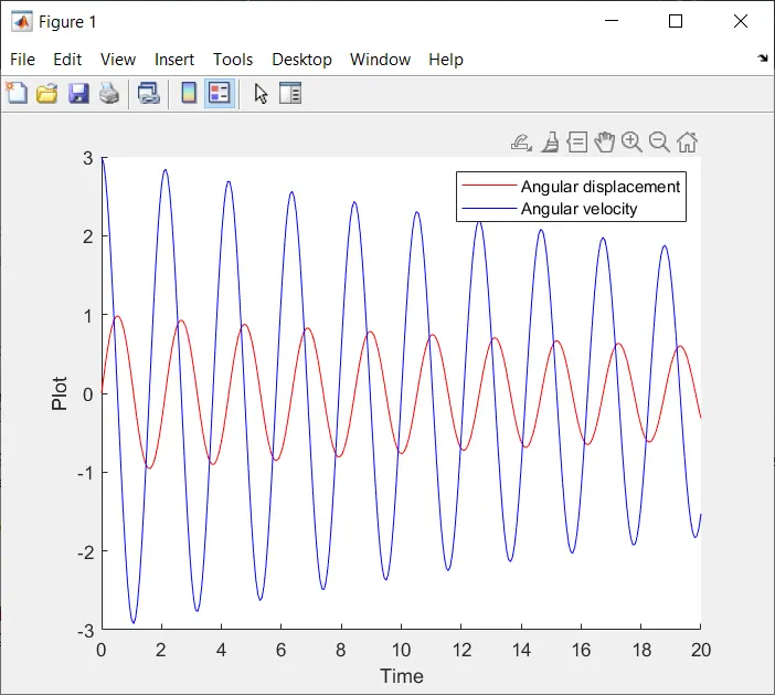
• Line-22: ---> Hold on command to show multiple plots in single figure
• Line-23: ---> Plotting t and angular displacement with colour of curve red.
• Line-24: ---> Plotting t and angular velocity with colour of curve blue.
• Line-25: ---> Labels X-axis of plot naming as Time (seconds).
• Line-26: ---> Labels Y-axis of plot naming as Plot.
• Line-27: ---> labelling the curves using legend command as Angular displacement and Angular velocity
• Line-31: ---> for loop starting from 1 to length of t.
• Line-33 to 37: ---> Giving coordinates of the pendulum as (x0,y0)=(0,0) and (x1,y1)= ( l*sin(results(i,1)) , -l*cos(results(i,1)) ) for each iteration of for loop as i runs from 1 to length of t.
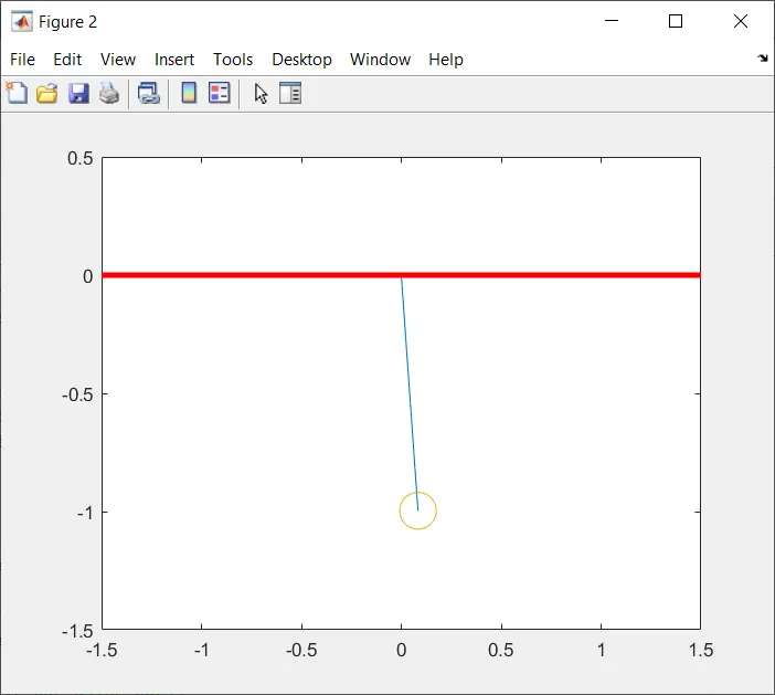
• Line-40: ---> Creating plots in another figure labeled as figure 2
• Line-41: ---> ploting a line between coordinates (x0,y0) and (x1,y1).
• Line-42: ---> Hold on command to show multiple plots in single figure.
• Line-43: ---> PLotting a line between coordinates (-1.5,0) and (1.5,0) of colour red and linewidth 3.
• Line-44: ---> Fixing the axis of plot between x-coordinates of -1.5 to 1.5 and y-coordinates -1.5 to 0.5.
• Line-45: ---> creating a circle at coordinates (x1,y1) of marker size 20 units for each iteration of for loop.
• Line-46: ---> Pausing the for loop for 0.0001 seconds.
• Line-47: ---> hold off command.
• Line-50: ----> Creating an Array (M) and store all the frames of the plot in the array.
• Line-51: ----> Increment of the variable (ct) by value 1 for each iteration.
• Line-52: ----> End of for loops.
• Line-54: ----> Creating a movie of array M.
• Line-55: ----> Creating a video file using VideoWriter command and labeling the video and its profile and storing the video in the variable 'videofile'.
• Line-56: ----> Opening the videofile.
• Line-57: ----> To create a video of all the frames in the array M.
• Line-58: ----> Close the videofile.

Output plots:

Errors faced while programming:

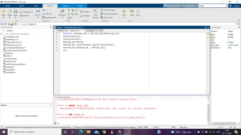
Output of function returns a colum matrix hence semicolon sholud be used in matrix dtheta_dt at line 6

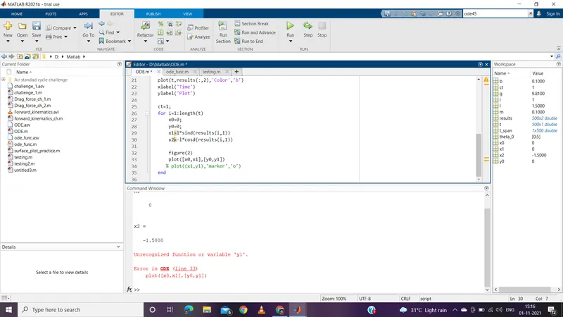
Proper usuage of variables on plot command according to the variable name.

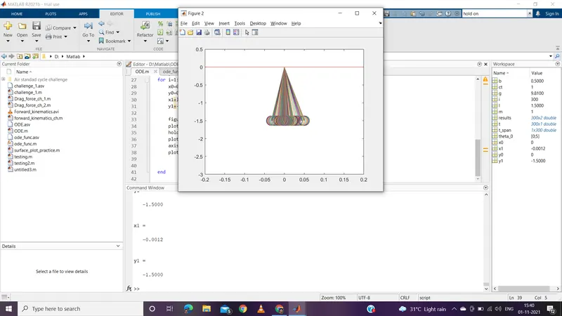
Proper usuage of hold on and hold off commands to avoid such errors or mistakes.

You-Tube link: https://youtu.be/jyQLigiJhHU