MATLAB CODE TO SIMULATE PENDULUM MOTION
MATLAB CODE TO SIMULATE PENDULUM MOTION
2nd Order Ordinary differential equation used:
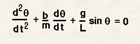
In the above equation,
g = gravity in m/s2,
L = length of the pendulum in m,
m = mass of the ball in kg,
b=damping coefficient.
Problem taken:
Write a program in Matlab that will simulate the pendulum motion
use,
L=1 metre,
m=1 kg,
b=0.05.
g=9.81 m/s2.
Simulate the motion between 0-20 sec, for angular displacement=0,angular velocity=3 rad/sec at time t=0.
MATLAB CODE:
% Matlab code to simulate pendulum motion
clear all
close all
clc

% inputs
b=0.05;  % damping coefficient
g=9.81;  % gravity in m/s2,
l=1;     % length of the pendulum in m,
m=1;     % mass of the ball in kg,

% initial conditions
theta_0=[0;3];

% time points
t_span=linspace(0,20,300);

% Solve ODE using ode45
[t,results]=ode45(@(t,theta) ode_func(t,theta,b,g,l,m),t_span,theta_0);

% Plotting Angular displacement and Angular velocity.
hold on
plot(t,results(:,1),'Color','r') % plot for Angular displacement
plot(t,results(:,2),'Color','b') % plot for Angular velocity
xlabel('Time')
ylabel('Plot')
legend('Angular displacement','Angular velocity')


ct=1;
for i=1:length(t)

    % Coordinates of pendulum with respect to angular displacement
    x0=0;
    y0=0;
    x1=l*sin(results(i,1))
    y1=-l*cos(results(i,1))

    % Plotting the pendulum movement.
    figure(2)
    plot([x0,x1],[y0,y1])
    hold on
    plot([-1.5 1.5],[0 0],'color','r','LineWidth',3)
    axis([-1.5 1.5 -1.5 0.5])
    plot(x1,y1,'o','MarkerSize',20)
    pause(0.0001)
    hold off

    % Capturing the frames
    M(ct)=getframe(gcf);
    ct=ct+1;
end
% Creating a video file
movie(M)
Videofile=VideoWriter('sec_order_ODE.avi','Uncompressed AVI')
open(Videofile)
writeVideo(Videofile,M)
close(Videofile)
FUNCTION CODE:
function [dthetha_dt] = ode_func(t,theta,b,g,l,m)

theta1=theta(1);        % Storing values of angular displacement
theta2=theta(2);        % Storing values of angular velocity

% Splitting 2nd order ODE
dtheta1_dt=theta2;
dtheta2_dt=-(b/m)*theta2-(g/l)*sin(theta1);

% Storing the values in variable
dthetha_dt=[dtheta1_dt ; dtheta2_dt];

end
CODE Explaination:
- Line-2: close all ----> closes all the Plots.
- Line-3: clear all ----> clears all the variables in the workspace.
- Line-4: clc ----> clears the command window.
- Line-6 to 10: ----> Inputs for the calculation. (As given in the problem)
- Line-13: ----> giving intitial conditions.
- Line-16: ----> Time span for the roblem to be solved.
- Line-19: ----> Using ode45 command,creating a anonymus function of variables (t,theta) and solving the ode_func whose inputs are (t,theta,b,g,l,m), and storing in the solutions in matrix [t,results]. Here results is an matrix of multiple rows and two columns storing the values of angular displacement in first column and angular velocity in second column with varying time. The time varied is stored in t which is a single column matrix. The function used is explained below
FUNCTION CODE:
- Line-1: ---> A function of name ode_func is made using function command with output variable [dthetha_dt] and input variables (t,theta,b,g,l,m).
- Line-3: ---> Storing values of angular displacement in variable theta1.
- Line-4: ---> Storing values of angular velocity in variable theta2.
- Line-7-8: ---> Splitting the 2nd order ODE into 1st order ODEs as dtheta1/dt = theta2 dtheta2/dt = -(b/m)*theta2-(g/l)*sin(theta1);
- Line-11: ---> Storing the values in variable dthetha_dt.
- Line-13: ---> end command to close the function.
- Line-21 to 27: ----> Plotting Angular displacement and Angular velocity Vs Time curves using plot command using the values of t and results two columns which represent Angular displacement and Angular velocity respectively. The xlabel for x-axies is givena as Time and ylabel for y-axis is given as Plot. legend ommand is used to distinguish the two curves inside the plot. The two curves are plotted on the same figure using hold on command.
- Line-31: ----> for loop to plot the motion of pendulum in a single frame.
- Line-33 to 37: ----> Giving the coordinates for the two end points of string as (x0,y0) and (x1,y1) for each iteration of for loop. The values of (x1,y1) can be calculated using formulae, x1=l*sin(results(i,1))
y1=-l*cos(results(i,1)) - Line-40: ----> Plots the upcomig plots in sepertate figure with label figure(2)
- Line-41: ----> Plotting line between coordinates (x0,y0) and (x1.y1).
- Line-42: ----> hold on command to not erase the previous plots.
- Line-43: ----> Plotting line between coordinates (-1.5,0) and (1.5,0) of colour red and width 3 units.
- Line-44: ----> Fixing the plot axis between x-coordinates=-1.5 to 1.5 and y-coordinates=-1.5 to 0.5.
- Line-45: ----> Creating a circle of size 20 at coordinates (x1,y1) for each iteration of for loop.
- Line-46: ----> Pausing the loop for about 0.0001 seconds.
- Line-47: ----> Putting off the hold on command.
- Line-50: ----> Creating an Array (M) and store all the frames of the plot in the array.
- Line-51: ----> Increment of the variable (ct) by value 1 for each iteration.
- Line-52: ----> End of for loop.
- Line-54: ----> Creating a movie of array M.
- Line-55: ----> Creating a video file using VideoWriter command and labeling the video as sec_order_ODE.avi and its profile as Uncompressed AVI and storing the video in the variable 'Videofile'.
- Line-56: ----> Opening the videofile.
- Line-57: ----> To create a video of all the frames in the array M.
- Line-58: ----> Close the videofile.
Output Figures:
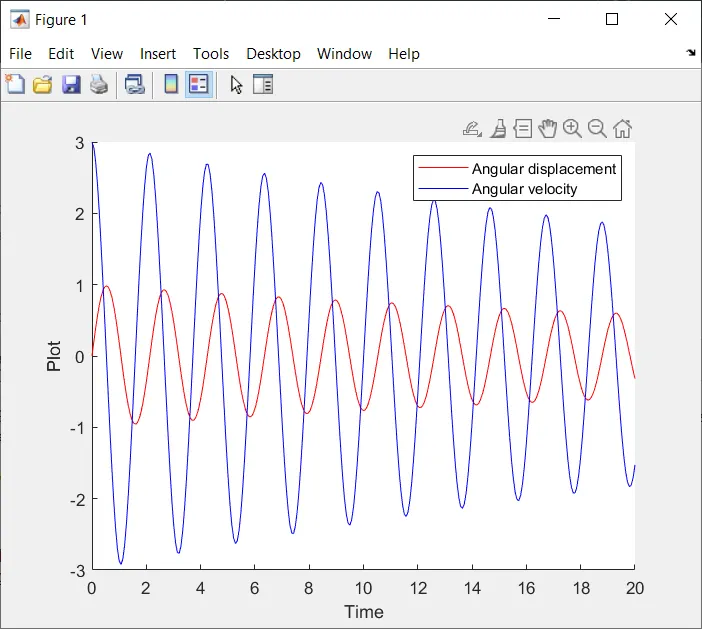
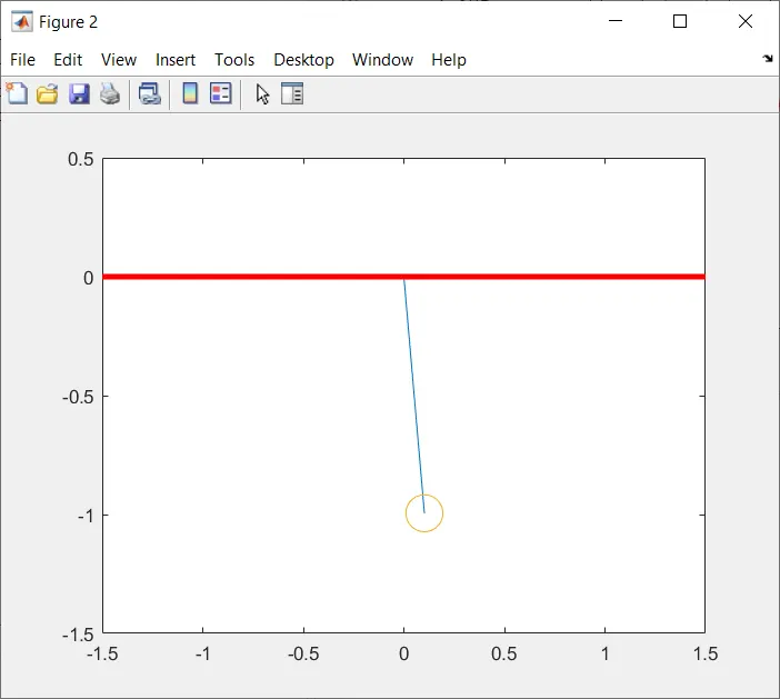
The motion of the pendulum is visible in form of video in you-tube link provided at the last part of report.
Errors faced while programming:
1.
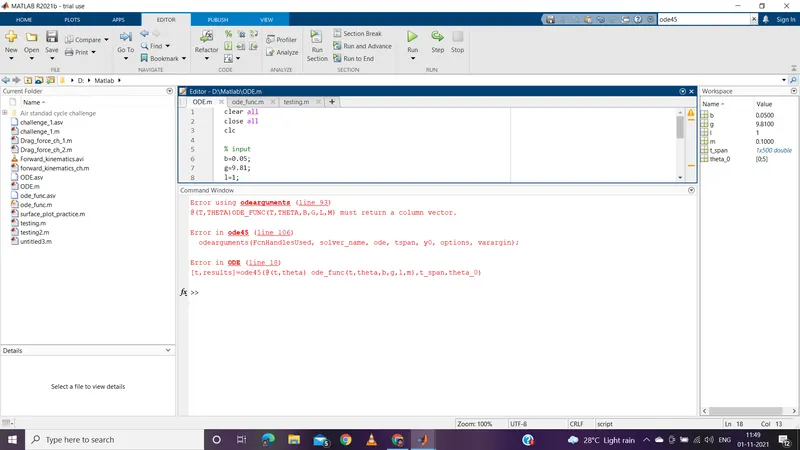
Made mistake in defining matrix of the ouput of function ode_func as it returns two columns.
2.
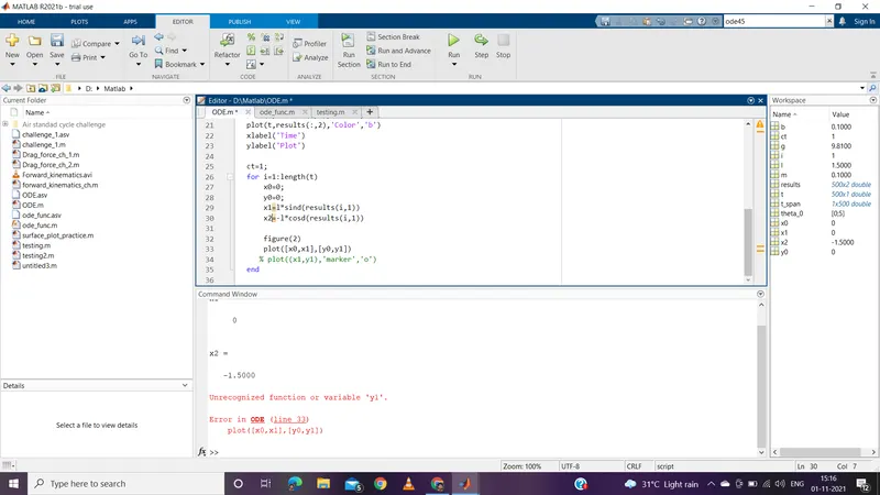
Made small mistake in defiining variables and using them.
3.
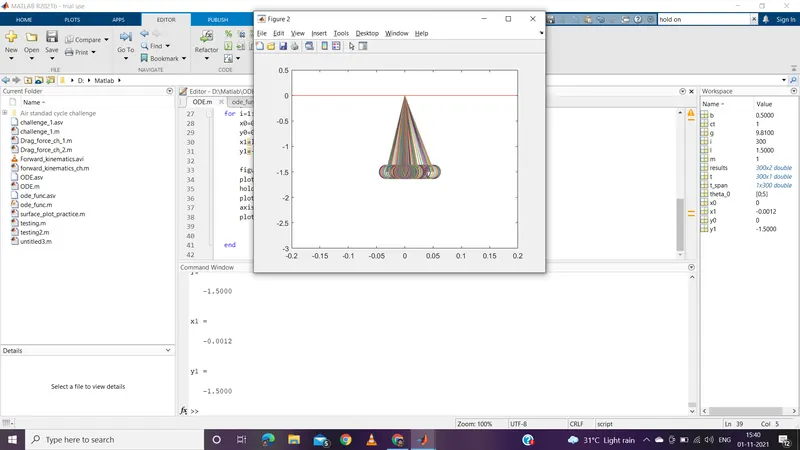
Made mistake in usuage of hold on and hold off commands.
4.
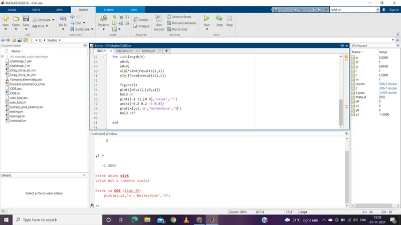
The numerical value for the size of marker sholud not e used under aphostrophes.
You-Tube Link: https://youtu.be/jyQLigiJhHU