Week 4.1 - Genetic Algorithm

Aim: To write code in MATLAB to optimise the stalagmite function and find the global maxima of the function.

Introduction:

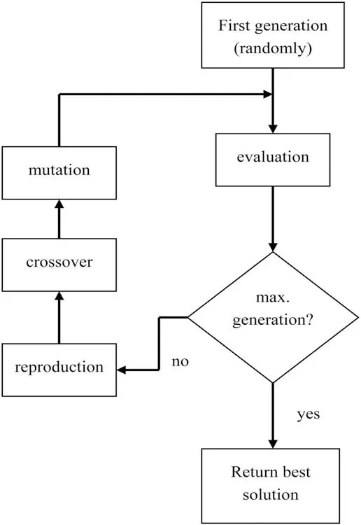
A genetic algorithm (GA) is inspired by Darwin's theory of evolution which states that the survival of an organism is affected by the rule "the strongest species that survives"and the process of natural selection that belongs to the larger class of evolutionary algorithm (EA).

Genetic algorithms are commonly used to generate high-quality solutions to optimization and search problems that are inspired by operators such as mutation, crossover & selection.

• Selection:

In this process, the fittest individuals are taken and pass their genes to the next generation.

Two pairs of individuals (parents) are selected based on their fitness scores. Individuals with high fitness have more chances to be selected for reproduction.

• Mutation:

In this process, random changes are performed to the parents to form the children for the next generation.

• Crossover

In this process, parents are to be mated to form children for the next generation.

• Program:

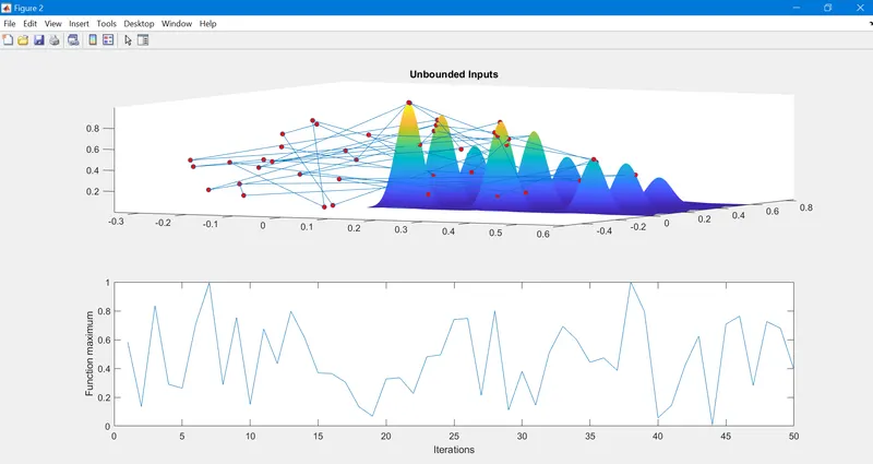
Here the program has 3- case studies as follows:

1) Study of genetic algorithm for random sampling.

In this, we run the ga() function and it takes random no.s as output and generates output beyond the search space.

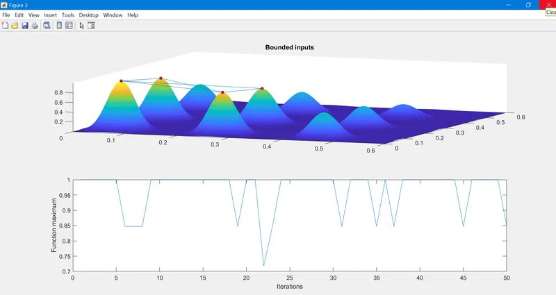
2) Study of genetic algorithm with upper and lower bounds.

In this, we specify the range of input variables to get the output in the desired fashion.

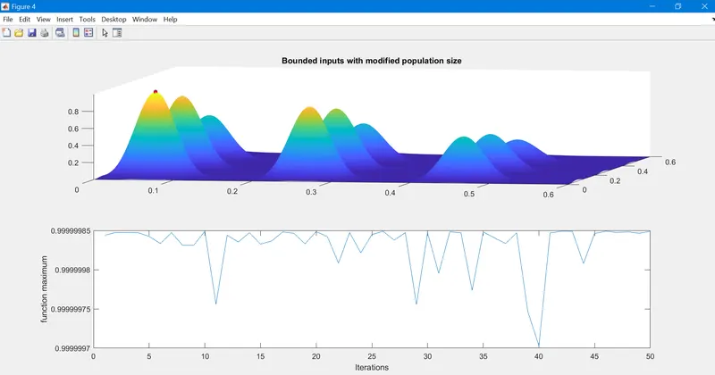
3) Study of genetic algorithm with upper and lower bounds and increase in the population size.

In the previous case, we are getting both the local and global maxima values. So in this study, we changed the initial population size along with the specified search space to get the maximum value with high probability as the aim of our program.

Note: Function ga() finds minimum value using genetic algorithm.

• Genetic algorithm ga() function syntax used in the program:

x=ga(@fun,nvars): where, 'fun' means function name & 'nvars' is the no. of variables.

x=ga(@fun,nvars,A,b,Aeq,beq): here, set of lower and upper bound is given so that the solution lies within the range.

x=ga(@fun,nvars,A,b,Aeq,beq,lb,ub,noncolon,intcon,options) where,

lb: lower bound;

ub: upper bound;

noncolon: non-linear constraints

intcolon: vector of positive integer

options: optimization option

Stalagmite:

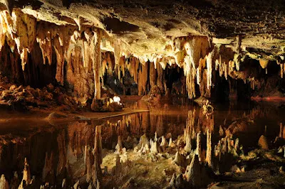
In general, a stalagmite is a type of rock formation that rises from the floor of a cave due to the accumulation of material deposited on the floor from ceiling drippings. Most stalagmites have rounded or flattened tips.

Use of the function stalagmite():-

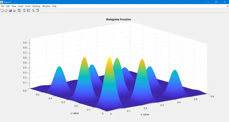
In the program, we have used the stalagmite function which helps to generate the local minima or maximas. The function predicts the minima value as shown in the below diagram.

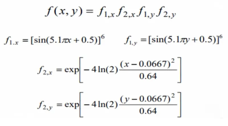
Defining the stalagmite function in matlab:

% stalagmite code



function [f]=stalagmite(input_vector)

x = input_vector(1);
y = input_vector(2);

f1_x = (sin(5.1*pi*x + 0.5))^6;
f1_y = (sin(5.1*pi*y + 0.5))^6;

f2_x = exp(-4*log(2) * ((x-0.0667)^2/0.64));

f2_y = exp(-4*log(2) * ((y-0.0667)^2/0.64));

f = -(f1_x*f1_y*f2_x*f2_y);

end

Note:

Here, we are using the (-) sign in f = -(f1_x*f1_y*f2_x*f2_y) as we have to calculate the maximum point for the optimization of GA as the aim of our program.

• Program to calculate the maximum value of stalagmite function using genetic algorithm:

clear all   %------clears the workspace
close all   %-------clears the figure window
clc   %------ clears the command window

% Inputs

% Defining the search space

x = linspace(0,0.6,150);  %---- creating 1-D array

y = linspace(0,0.6,150);  %----- creating 1-D array

% Creating a 2-D mesh

[XX,YY] = meshgrid(x,y);

% To evaluate the stalagmite function

for i = 1:length(XX) 

    for j = 1:length(YY)

        input_vector(1)=XX(i,j); %--- assigning value of XX(i,j) array element to input_vector(1) 

        input_vector(2)=YY(i,j); %---assigning value of YY(i,j) array element to input_vector(2)

    f(i,j)= stalagmite(input_vector);  %--- calling the function & assigning th value of (i,j)

    end
end

%Plotting

figure(1) %---- indicates the figure of stalagmite function

surfc(XX,YY,-f)  %--- creates a three-dimensional surface plot with a contour plot underneath
title('Stalagmite Function')
xlabel('x value')
ylabel('y value')

shading interp  % --- makes the plot smoother

[inputs,fval]=ga(@stalagmite,2);


% Statistical behaviour*******


num_case = 50; % ---- no. of iterations

tic % ---- to record the current time

for i = 1:num_case

    [inputs, fopt(i)]=ga(@stalagmite,2); % ---- to find the minimum value using ga function and assigning the optimized value to fopt & assigning the value to inputs array to which we got the minimum value 

    xopt(i) = inputs(1);
                         % ----- storing the values of x,y
    yopt(i) = inputs(2);

end

study1_time = toc; % ---- to measure the elapsed time

figure(2) % --- figure of unbounded inputs

subplot(2,1,1)  %---- creates multiple plot inside the same figure window

hold on 
surfc(x,y,-f) %--- creates a three-dimensional surface plot with a contour plot underneath

shading interp

plot3(xopt,yopt,-fopt,'marker','o','markersize',5,'MarkerFaceColor','r') %--- plotting the optimized maximum value which we got from ga() in unbounded case

title('Unbounded Inputs')

subplot(2,1,2)

plot(-fopt) %---plotting the function maximum vs iteration
xlabel('Iterations')
ylabel('Function maximum')

% Statistical behaviour with upper & lower bounds******

tic %---- to record the current time

for i = 1:num_case

    [inputs,fopt(i)]=ga(@stalagmite,2,[],[],[],[],[0,0],[0.6,0.6]); % --- fixing upper & lower bounds

    xopt(i)=inputs(1);
                       %----- storing the  value for x & y
    yopt(i)=inputs(2);

end

study2_time=toc %---- to measure the elapsed time

figure(3) %-- figure of bounded inputs
subplot(2,1,1)
hold on
surfc(x,y,-f) % ----creates a three-dimensional surface plot with a contour plot underneath
shading interp

plot3(xopt,yopt,-fopt,'marker','o','markersize',5,'markerfacecolor','r')

title('Bounded inputs')

subplot(2,1,2) %--- creating the subplot for plotting the function maximum vs iteration

plot(-fopt) %---- plotting the function maximum vs iteration
xlabel('Iterations')
ylabel('Function maximum')


% Study 3 increasing the GA iterations

options = optimoptions('ga');
options = optimoptions(options,'PopulationSize',230); 

tic %---- to record the current time

for i = 1:num_case

    [inputs,fopt(i)]=ga(@stalagmite,2,[],[],[],[],[0,0],[0.6,0.6],[],[],options);

    xopt(i)=inputs(1);
                      % storing values for x & y
    yopt(i)=inputs(2);

end

study3_time = toc %----- to measure the elapsed time

figure(4)
subplot(2,1,1) %--- creating subplot for 3-D surface
hold on
surfc(x,y,-f) %---- creates a 3-D surface plot with a contour plot underneath
shading interp %--- makes the plot smoother
plot3(xopt,yopt,-fopt,'marker','o','markersize',5,'markerfacecolor','r') %--- plotting the optimized maximum value (-fopt) bounded inputs with population size of 230

title('Bounded inputs with modified population size')
subplot(2,1,2) %---- creating the subplot for plotting the function maximum vs iteration
plot(-fopt) %---- plotting the function maximum vs iteration
xlabel('Iterations')
ylabel('function maximum')

• OUTPUTS:

• Stalagmite function

• Study-1: GA for the random & unbounded sampling

• Study-2: GA with upper & lower bound sampling

• Study-3: GA with upper & lower bound and increase in population size

Conclusion:

By using genetic algorithm, we are able to get the global maxima point of a stalagmite function. The function ga() predicts the minimum value but we have put the (-) negative sign in the function '-f' also '-fopt' everywhere in the program to get the global maxima. It can be observed from study-3 that we have achieved the global maxima point with an increase or modified population size of 230. The study time increases as an increase in the population size to get more accurate results.

• Error faced in the programming:

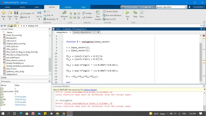
Error: Local function name must be different from the script name.

Correction: To create a function, it is not required to start with close all, clear all & clc commands as by-mistake I was getting the error, so removed the commands from lines no.1,2 &3.