Week 3 - Solving second order ODEs

Aim: To solve 2nd order ODE by an example of 'Simple Pendulum'.

Objective: To write a program that solves the following ODE. This ODE represents the equation of motion of a simple pendulum with damping

In the above equation,

g = gravity in m/s2,

L = length of the pendulum in m,

m = mass of the ball in kg,

b=damping coefficient.

Defined parameters are as:

L=1 metre,

m=1 kg,

b=0.05.

g=9.81 m/s2.

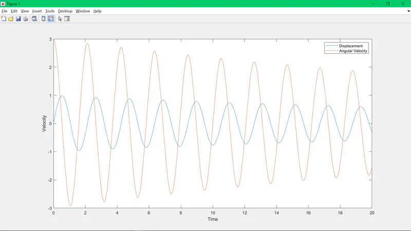
Simulate the motion between 0-20 sec, for angular displacement=0,angular velocity=3 rad/sec at time t=0.

#Program that solves the ODE represents the equation of motion of a simple pendulum with damping

clear all
close all
clc


% To solve the ODE represents the equation of motion of a simple pendulum with damping

% Inputs

% g = gravity in (m/s^2)

g = 9.81;

% l = length of pendulum (meter)

l = 1;

% mass of ball in (kg)

m = 1;

% b = damping coefficient

b = 0.05;

% Initial condition for displacement & velocity

theta_0 = [0;3]; 

% Timepoints

t_span = linspace(0,20,500);

% To solve ODE

% Here ode45 is an inbuild solver for nonstiff differential equations used in Matlab

[t,results] = ode45(@(t,theta) ode_func(t,theta,b,g,l,m),t_span,theta_0);

figure(1)

plot(t,results(:,1)) % Angular displacement

hold on

plot(t,results(:,2)) % Angular velocity

xlabel('Sec')

ylabel('Rad/sec')

legend('Angular Displacement','Angular Velocity')


ct=1; % counter represents each and every frame

for i= 1:length(t)

    % Fixing the coordinates where the pendulum rod is attached
     x0=0;
     y0=0;

    % Resolving the FBD of the pendulum ball

    x1= l*sin(results(i,1));
    y1= -l*cos(results(i,1));

    figure(2)

    % Plotting the massless pendulum rod
    plot ([x0 x1],[y0 y1],'color','b');

    hold on

    % Plotting the horizontal support for the pendulum
   
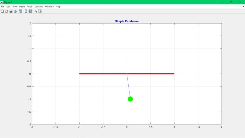
    line ([-1 1], [0 0], 'linewidth',4,'color','r');

    hold on

    plot(x0,y0,'marker','o','markersize',3,'markerfacecolor','y') % for the pivot where pendulum rod attached

    
    plot(x1,y1,'marker','o','markersize',20,'markerfacecolor','g') % for the pendulum ball

    % defining the axis

    axis([-2 2 -2 2])

   grid on

  % captures the current axes as it appears on the screen as a movie frame.
   M(ct)=getframe(gcf); 
   pause(0.02);

   ct=ct+1;
   hold off
   
end

movie(M) % Creating a movie of variable 'M' which contains all frame
videofile = VideoWriter('Simple_pendulum_animation.avi'); %Creating videofile with specified format 
open(videofile) % To open the video file for writting
writeVideo(videofile,M) % to write video data to an AVI file with Motion JPEG compression.
close(videofile)

• ODE45:

Integrates the system of differential equations with initial to the final condition. Each row in the solution array corresponds to a value returned in the column vector.

% Program to call the ODE function in SHM

function [dtheta_dt] = ode_func(t,theta,b,g,l,m)

theta1 = theta(1);
theta2 = theta(2);
dtheta1_dt = theta2;
dtheta2_dt = -(b/m)*theta2 - (g/l)*sin(theta1);
dtheta_dt = [dtheta1_dt;dtheta2_dt];
end

Output 1:

Output 2:

Errors faced during the program:

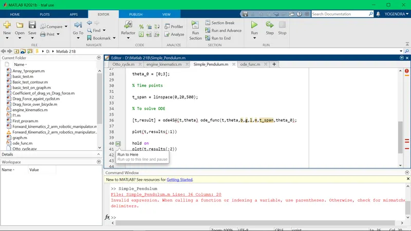
Error faced: The code was getting an error due to parentheses was missing.

Correction done: After ode45 '(' was missing, so corrected.

Conclusion: As we have studied the transient motion of a simple pendulum with damping by solving 2nd order ODE on 'MATLAB' that can be checked & analysed with the help of plots and animation.

• Youtube link for the animation of Simple pendulum: https://www.youtube.com/watch?v=HGCFviREb9o