Week 4.1 - Genetic Algorithm
AIM:
- MATLAB code to optimise the stalagmite function and find the ‘global maxima’ of the function.
- Plot graphs for all the studies for ‘maximum value of function’ vs ‘no. of Iterations’
Objectives:
- Need for optimization
- Concept of ‘genetic algorithm’ and its syntax in MATLAB
- Stalagmite function
- Compare all the studies in this session and provide a conclusion.
Introduction to Optimization
Optimization is the process of making something better. In any process, we have a set of inputs and a set of outputs as shown in the following figure.
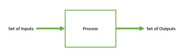
- Optimization refers to finding the values of inputs in such a way that we get the “best” output values.
- The definition of “best” varies from problem to problem, but in mathematical terms, it refers to maximizing or minimizing one or more objective functions, by varying the input parameters.
- The set of all possible solutions or values which the inputs can take make up the search space. In this search space, lies a point or a set of points which gives the optimal solution. The aim of optimization is to find that point or set of points in the search space.
Techniques available to perform optimization:
Deterministic method: They use specific rules for moving one solution to another. In this technique, the output of the model is fully determined by the parameter values and the initial conditions.
Example: Stress analysis of the component
Stochastic method: These are gaining popularity due to certain properties which deterministic algorithms do not possess. Stochastic models possess some inherent randomness, it is a probabilistic approach.
Example: Varying the water paths from the mountain can vary the regional weather conditions.
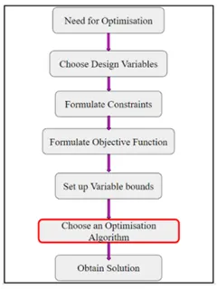
The following is the procedure followed by any optimization process:
Genetic Algorithms:
Genetic algorithms are based on the ideas of natural selection and genetics. These are intelligent exploitation of random search provided with historical data to direct the search into the region of better performance in solution space.
They are commonly used to generate high-quality solutions for optimization problems and search problems.
Genetic algorithms simulate the process of natural selection which means those species who can adapt to changes in their environment are able to survive and reproduce and go to next generation. In simple words, they simulate “survival of the fittest” among individual of consecutive generation for solving a problem.
Genetic algorithms are based on an analogy with genetic structure and behaviour of chromosomes of the population. Following is the foundation of GAs based on this analogy:
- Individual in population compete for resources and mate
- Those individuals who are successful (fittest) then mate to create more offspring than others
- Genes from “fittest” parent propagate throughout the generation, that is sometimes parents create offspring which is better than either parent.
- Thus, each successive generation is more suited for their environment
Fitness Score:
A Fitness Score is given to each individual which shows the ability of an individual to “compete”. The individual having optimal fitness score (or near optimal) are sought.
The individuals having better fitness scores are given more chance to reproduce than others. The individuals with better fitness scores are selected who mate and produce better offspring by combining chromosomes of parents.
Each new generation has on average more “better genes” than the individual (solution) of previous generations. Thus, each new generations have better “partial solutions” than previous generations.
Once the off-springs produced having no significant difference than offspring produced by previous populations, the population is converged. The algorithm is said to be converged to a set of solutions for the problem.
Operators of Genetic Algorithms:
Once the initial generation is created, the algorithm evolves the generation using following operators:
- Selection Operator: The idea is to give preference to the individuals with good fitness scores and allow them to pass their genes to successive generations.
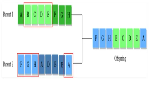
- Crossover Operator: This represents mating between individuals. Two individuals are selected using selection operator and crossover sites are chosen randomly. Then the genes at these crossover sites are exchanged thus creating a completely new individual (offspring). For example –
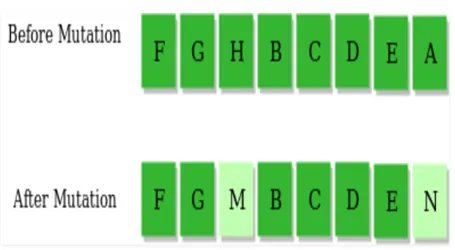
- Mutation Operator: The key idea is to insert random genes in offspring to maintain the diversity in the population to avoid premature convergence. For example –
The whole algorithm can be summarized as –
1) Randomly initialize populations
2) Determine fitness of population
3) Until convergence repeat:
a) Select parents from population
b) Crossover and generate new population
c) Perform mutation on new population
d) Calculate fitness for new population
Some of the genetic algorithm applications:
- Natural Sciences, Mathematics and Computer Science
- Earth Sciences
- Finance and Economics
- Social Sciences
- Industry, Management and Engineering
‘Genetic algorithm’ syntax in MATLAB:
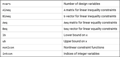
x = ga(fun,nvars) à (finds a local unconstrained minimum, x, to the objective function, fun. nvars is the dimension (number of design variables) of fun.)
x = ga(fun,nvars,A,b) à (finds a local minimum x to fun, subject to the linear inequalities A*x ≤ b. ga evaluates the matrix product A*x as if x is transposed (A*x').
x = ga(fun,nvars,A,b,Aeq,beq) à ( finds a local minimum x to fun, subject to the linear equalities Aeq*x = beq and A*x ≤ b. (Set A=[] and b=[] if no linear inequalities exist.) ga evaluates the matrix product Aeq*x as if x is transposed (Aeq*x').)
x = ga(fun,nvars,A,b,Aeq,beq,lb,ub) à (defines a set of lower and upper bounds on the design variables, x, so that a solution is found in the range lb ≤ x ≤ ub. (Set Aeq=[] and beq=[] if no linear equalities exist.))
x = ga(fun,nvars,A,b,Aeq,beq,lb,ub,nonlcon) à (subjects the minimization to the constraints defined in nonlcon. The function nonlcon accepts x and returns vectors C and Ceq, representing the nonlinear inequalities and equalities respectively. ga minimizes the fun such that C(x) ≤ 0 and Ceq(x) = 0. (Set lb=[] and ub=[] if no bounds exist.))
x = ga(fun,nvars,A,b,Aeq,beq,lb,ub,nonlcon,options) à ( minimizes with the default optimization parameters replaced by values in options. (Set nonlcon=[] if no nonlinear constraints exist.) Create options using optimoptions.)
x = ga(fun,nvars,A,b,Aeq,beq,lb,ub,nonlcon,intcon) or
x = ga(fun,nvars,A,b,Aeq,beq,lb,ub,nonlcon,intcon,options) à (requires that the variables listed in intcon take integer values.)
x = ga(problem) à (finds the minimum for problem, a structure described in problem.)
[x,fval] = ga(___) à (for any previous input arguments, also returns fval, the value of the fitness function at x.)
[x,fval,exitflag,output] = ga(___) à (also returns exitflag, an integer identifying the reason the algorithm terminated, and output, a structure that contains output from each generation and other information about the performance of the algorithm.)
[x,fval,exitflag,output,population,scores] = ga(___) à (also returns a matrix population, whose rows are the final population, and a vector scores, the scores of the final population.)
Stalagmite function:
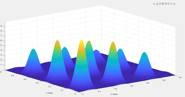
A stalagmite is an upward-growing mound of mineral deposits that have precipitated from water dripping onto the floor of a cave. Most stalagmites have rounded or flattened tips. There are many other types of mineral formations found in caves. Another example is the icebergs in the oceans.
Mathematical equation to represent stalagmite is as follows:
f(x,y) = f1,x f2,x f1,y f2,y
where as:
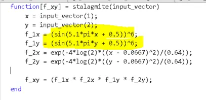
f1,x = [sin(5.1πx + 0.5)]6
f1,y = [sin(5.1πy + 0.5)]6
f2,x = exp[- 4ln(2) (x - 0.0667)2/(0.64)]
f2,y = exp[- 4ln(2) (y - 0.0667)2/(0.64)]
MATLAB code to optimise the stalagmite function and find the ‘global maxima’ of the function
Function code:
%% Stalagmite Function%%
%% f_xy = (f_1x * f_2x * f_1y * f_2y) is the equation for caluculating the stalagmite function.
%% By using 'ga' command the minimum value of a function is provided as output generally.
%% In this function, we have modified the stalagmite equation by adding a negative sign infront of it.
%% In this way when the 'ga' is executed the minimum value will be provided as output which is in this case
%% can be considered as the maximum value, that we are interested in.

function[f_xy] = get_stalagmite(input_vector)
    x = input_vector(1);
    y = input_vector(2);
    f_1x = (sin(5.1*pi*x + 0.5))^6;
    f_1y = (sin(5.1*pi*y + 0.5))^6;
    f_2x = exp(-4*log(2)*((x - 0.0667)^2)/(0.64));
    f_2y = exp(-4*log(2)*((y - 0.0667)^2)/(0.64));

    f_xy = -(f_1x * f_2x * f_1y * f_2y);
end
Main code:
%%%% GENETIC ALGORITHM %%%%
clear all
close all
clc

% Inputs to create 2D array
x = linspace(0,0.6,150);
y = linspace(0,0.6,150);
num_cases = 50; % No. of iterations for GA

% Creating 2D array using x and y. This is the search space.
[xx, yy] = meshgrid(x,y);

% Evaluating the Stalagmite function, the output data of this function is
% used to create a surface plot
for i = 1:length(xx)
    for j = 1:length(yy)
        input_vector(1) = xx(i,j);
        input_vector(2) = yy(i,j);
        f(i,j) = get_stalagmite(input_vector);
    end
end

%% Study 1 - Statistical behaviour with 'Unbounded inputs'
tic  %start of the timer
for i = 1: num_cases
    [inputs, fopt(i)] = ga(@get_stalagmite,2); %% since there are 2 varaibles in this case (xx(i,j) and yy(i,j)
    % xopt and yopt are the optimum values at which the function has a maximum value.
    xopt(i) = inputs(1);
    yopt(i) = inputs(2);
end
Study_1_time = toc % end of the timer

figure(1)
subplot(2,1,1) % Multiple plots in a same figure window; Create axes in tiled positions
hold on
surfc(xx,yy,f)
xlabel('x-axis');
ylabel('y-axis');
zlabel('Function values')
shading interp  %% Removes the gridlines on the plot and enable shading
plot3(xopt,yopt,fopt, 'marker','o', 'markersize',8,'markerfacecolor','r'); % plot3(X,Y,Z) plots coordinates in 3-D space.
title('Unbounded inputs')
subplot(2,1,2) % Multiple plots in a same figure window; Create axes in tiled positions
plot(fopt) % Plotting the function values vs Iterations
xlabel('No. of Iterations')
ylabel('Function maximum')

%% Study 2 - Statistical behaviour - with upper and lower bounds
tic  %start of the timer
for i = 1: num_cases
    [inputs, fopt(i)] = ga(@get_stalagmite,2,[],[],[],[],[0;0],[0.6;0.6]); % defining upper and lower bounds of inputs here, refer syntax
    xopt(i) = inputs(1);
    yopt(i) = inputs(2);
end
Study_2_time = toc;  %end of the timer

figure(2)
subplot(2,1,1)
hold on
surfc(xx,yy,f)
xlabel('x-axis');
ylabel('y-axis');
zlabel('Function values')
shading interp
plot3(xopt,yopt,fopt, 'marker','o', 'markersize',8,'markerfacecolor','r');
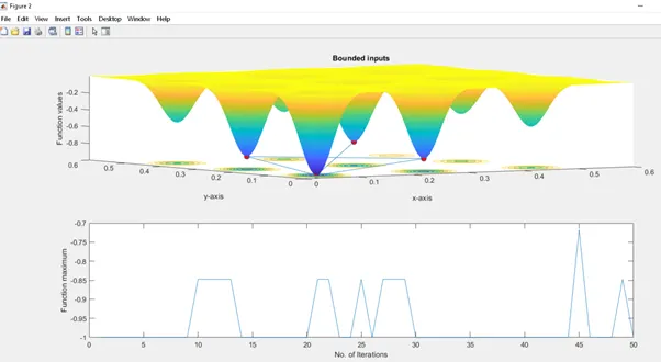
title('Bounded inputs')
subplot(2,1,2)
plot(fopt)
xlabel('No. of Iterations')
ylabel('Function maximum')

%% Study 3 - Increasing GA iterations

% options is used in in 'ga' command, to replace the  initially defined number of iterations
options = optimoptions('ga');
options = optimoptions(options, 'PopulationSize',200)

tic   %start of the timer
for i = 1: num_cases
    [inputs, fopt(i)] = ga(@get_stalagmite,2,[],[],[],[],[0;0],[0.6;0.6],[],[],options);
    xopt(i) = inputs(1);
    yopt(i) = inputs(2);
end
Study_3_time = toc;  %end of the timer

figure(3)
subplot(2,1,1)
hold on
surfc(xx,yy,f)
xlabel('x-axis');
ylabel('y-axis');
zlabel('Function values')
shading interp
plot3(xopt,yopt,fopt, 'marker','o', 'markersize',8,'markerfacecolor','r');
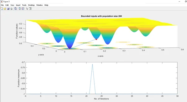
title('Bounded inputs with population size 200')
subplot(2,1,2)
plot(fopt)
xlabel('No. of Iterations')
ylabel('Function maximum')

%% Study 4 - Increasing GA iterations further more

% options is used in in 'ga' command, to replace the  initially defined number of iterations
options = optimoptions('ga');
options = optimoptions(options, 'PopulationSize',500)

tic   %start of the timer
for i = 1: num_cases
    [inputs, fopt(i)] = ga(@get_stalagmite,2,[],[],[],[],[0;0],[0.6;0.6],[],[],options);
    xopt(i) = inputs(1);
    yopt(i) = inputs(2);
end
Study_4_time = toc;  %end of the timer

figure(4)
subplot(2,1,1)
hold on
surfc(xx,yy,f)
xlabel('x-axis');
ylabel('y-axis');
zlabel('Function values')
shading interp
plot3(xopt,yopt,fopt, 'marker','o', 'markersize',8,'markerfacecolor','r');
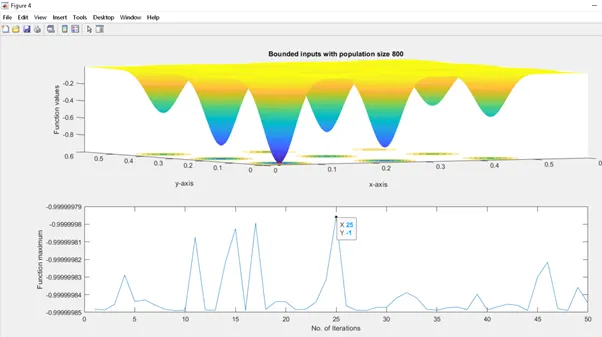
title('Bounded inputs with population size 800')
subplot(2,1,2)
plot(fopt)
xlabel('No. of Iterations')
ylabel('Function maximum')
Output:
Study 1 plot:
Study 2 plot:
Study 3 plot:
Study 4 plot:
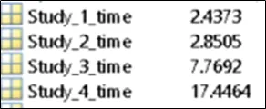
Time taken for each study:
Explanation of the code:
- Initially, a search space is created where the ‘ga’ gets the inputs from using meshgrid command.
- Using the ‘stalagmite function’ code, the values of that function are calculated by taking the 2D array coordinates as input (see above step)
- GA in matlab minimizes a function in MATLAB, but in this session since we are interested to find the maximum point of the function, we have modified the stalagmite equation by adding a negative sign infront of it. In this way when the 'ga' is executed the minimum value will be provided as output which is in this case can be considered as the maximum value.
- Four studies have been created for this case to see how we can get the maximum point of the function by limiting the inputs and increasing the iteration size. By doing this iterative process, the function is converged and a maximum point of the function is calculated.
- Using the ‘ga’ command the ‘stalagmite function’ and ‘number of variables’ are called. The output of this command are two things:
- Optimum value of a given function.
- The x and y coordinates where the given function is optimum.
- In all the studies a sub-plot has been created to visualize multiple plots in a single figure window.
- In a particular figure, two graphs have been plotted:
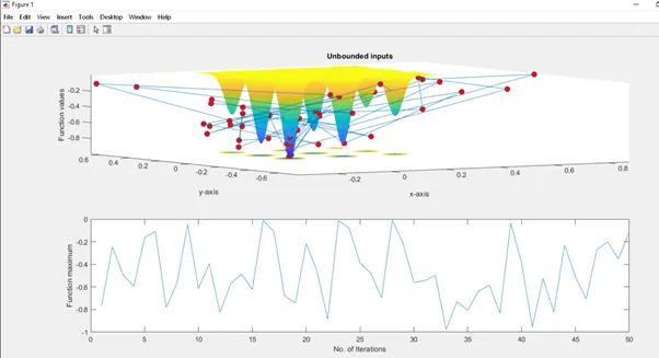
- a surface plot using ‘2D array inputs and function’ along with ‘optimum values of inputs and functions’ are plotted in one graph.
- A plot where the ‘function values’ vs ‘No. of iterations’ is plotted.
Observations made from the four studies:
- In the first study, where the inputs were unbounded (the x and y values were going away from the defined limits 0 and 0.6), the maximum value of the function varies in each iteration and the variation is from 0 to -1.
- In the second study, the inputs were bounded between 0 and 0.6 and the result is the maximum function values are optimized compared to study 1. The maximum value of the function varies in between 3 points.
- In the third study, the inputs were bounded same as study 2 but with an increased population size of 200(compared to 50 in study 1 and 2). Here we could able to see the maximum value of the function is varying between 2 points.
- In the fourth study, the inputs were bounded same as study 2 but with an increased population size of 800(compared to 200 in study 3). Here we could able to see the maximum value of the function is fixed at one point and this is the value we want.
- The time taken for all these studies is recorded and we can see that the time taken to execute each study is different and increasing with increase in population size.
Conclusion:
From the above studies we can conclude that ‘ga’ can be used to find maximum value of the ‘stalagmite function’ as well. By constraining the inputs and increasing the population size ‘ga’ can converge towards a more optimized solution.
References:
https://skill-lync.com/knowledgebase/genetic-algorithm-explained
https://mech.iitm.ac.in/nspch52.pdf
https://www.tutorialspoint.com/genetic_algorithms/genetic_algorithms_introduction.htm
https://www.geeksforgeeks.org/genetic-algorithms/
https://en.wikipedia.org/wiki/Genetic_algorithm
https://en.wikipedia.org/wiki/List_of_genetic_algorithm_applications
https://in.mathworks.com/help/matlab/ref/subplot.html?s_tid=doc_ta
https://in.mathworks.com/help/matlab/ref/plot3.html?searchHighlight=plot3&s_tid=srchtitle_plot3_1
Errors:
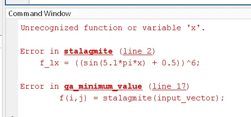
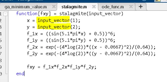
1. The variable x and y for the stalagmite function were not defined, hence the error:
Resolved it by providing the inputs as shown:
2. Wrong equation in the Stalagmite function leading to incorrect surface plot
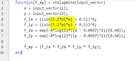
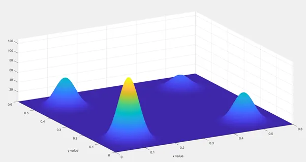
Resolution: Corrected the equation as shown and could able to get the right plot