Week 3 - Solving second order ODEs

AIM:

1. Execute a MATLAB program to solve 2^nd order ODE which demonstrated a simple pendulum with damping.
2. Create an animation of simple pendulum with damping

Introduction:

In engineering, ODE is used to describe the transient behaviour of a system.

The way a simple pendulum moves depends on the Newtons second law.

Newton's second law: An object at rest stays at rest, and an object in motion will stay in motion, at a constant speed in a straight line, unless another force acts upon it. The acceleration of an object depends on the mass of the object and the amount of force applied.

ODE that represents the motion of a simple pendulum with damping is defined by following equation:

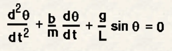
This equation describes the position of the 'ball' with respect to time.

where as:

g = gravity (m/s^2)

L = length of the pendulum (m)

m = mass of the ball (Kg)

b = damping coefficient

MATLAB CODE:

clear all
close all
clc

%inputs
l = 2; %length of the pendulum (m)
m = 1; %mass of the ball (Kg)
g = 9.81; % gravity (m/s^2)
b = 0.05; % damping coefficient

%initial condition
disp_vel = [0;3];  %Here displacement = 0 and Velocity = 3 m/s

%timepoints (These are inegration limits)
t_span = [0,20]; % The solver will choose a step size that is most suitable for the solution in the most optimal time

% solving ODE, ode is a function of t and y. ode_func gives the results of
% displacement and velocity. The results would be an array of optimum no. of rows to 2 columns.

[t, results] = ode45(@(t,y) ode_func(t,y,b,g,l,m), t_span, disp_vel);

%Plotting
figure(1)
plot(t, results(:,1)) % this curve gives time vs displacement
hold on
plot(t,results(:,2))  % this curve gives time vs velocity
xlabel('time')
ylabel('plot')
legend('Angular Displacement', 'Angular velocity') % To identify the plot

%Creating an animation for motion of simple pendulum with damping

ct = 1; % Counter: ct represents frame number here
for i = 1:length(results(:,1))

% Considering a fixed point --> in this case origin.
    a0 = 0;
    b0 = 0;
% The coordinates which the ball is tracing can be represented by length multiplied by sin and cos of the position at a given time.
    a1 = l*sin(results(i,1));
    b1 = -l*cos(results(i,1)); % negative sign is added here, just to make the plot look realistic.

    figure(2)
    plot([a0,a1], [b0,b1], 'linewidth', 2, 'Marker','O')
    axis([-4 4 -4 4]);
    axis off
    

% M is an array which is going to save the figures/frames
        % ct represents frame number here and gcf --> current figure window
        M(ct) = getframe(gcf); 
        ct = ct+1;  
end

movie(M)
Videofile = VideoWriter('Simple_pendulum.avi', 'Uncompressed AVI');  % Name of the video file
open(Videofile);          % Open the video file
writeVideo(Videofile,M);  % writing the movie in the video file
close(Videofile);         % closing the video file

Function used:

function[dy_dt] = ode_func(t,y,b,g,l,m)

dydt(1) = y(2);  % 
dydt(2) = -(b/m)*y(2) - (g/l)*sin(y(1));
dy_dt = [dydt(1); dydt(2)];

end

Explanation of the code:

Initially we are assuming the length of the pendulum, mass of the ball and damping coefficient.

Also, the initial conditions of displacement and velocity are considered. The time span between 0 to 20 seconds is considered to check the displacement and velocity at each step between this time interval.

Using the ODE45 command the first order ODE equations are solved and the results are plotted w.r.t time.

Here the ODE45 needs 3 inputs which are: function to be integrated, time span and initial conditions.

Providing legend command to identify the plots.

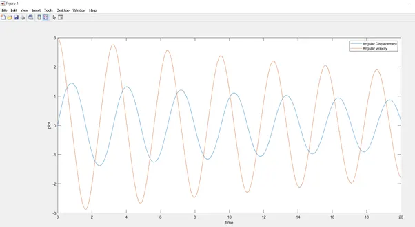
From the above plot it can be seen that the pendulum started with a velocity of 3 m/s and gradually it is been decreasing.

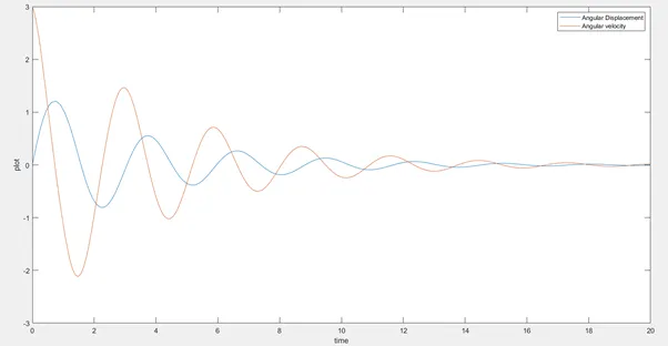
If the damping coefficient is increased, let us take b = 0.5, and run the code, we can see in the below plot that the motion of the pendulum is been damping out quickly right after half the time span and bringing the ball to rest position.

An animation is created to demonstrate this motion and the comments are mentioned in the code.

To plot the animation that gives a more realistic view is by using the plot command and storing the frames by using 'getframe' command. The frames are stored in a array form and this will be the input for 'movie' command. The video file is generated by using the commands: Videofile, VideoWriter, open(Videofile), writeVideo, close.

The animation is present in below path:

https://drive.google.com/file/d/1S4TB-cRIivY8I1wNbo2d2zMSvTUCgz2r/view?usp=sharing

Function used in the main program:

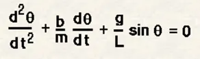
consider θ = y(1) --> Angular displacement

dθ/dt = dy(1)/dt = y(2) --> Angular velocity

d²θ/dt² = -(b/m)*y(2) - (g/l)*sin(y(1))

Here we are breaking the second order ODE into first order ODE, because MATLAB can only solve first order ODE. This function will provide the output as displacement in first column and velocity in second column for each step of time.

Error:

I have used following code to animate:

t_span1 = linspace(0, 20, 120)

vel= results(:,2);

ct = 1;

 

for i = 1:20 

    vel1= vel(i);

      for j = 1:120

          t1 = t_span1(i);

 

        %initial condition

        t0 = 0;                

        vel0 = 0 ;               

 

        %plotting

        plot([t0 t1],[vel0 vel1], 'linewidth', 2, 'Marker','o')

        axis([-30 30 -30 30] )

%         pause(0.00000001)

       

        % M is an array which is going to save the figures/frames

        % ct represents frame number here and gcf --> current figure window

        M(ct) = getframe(gcf);

        ct = ct+1; 

       

       end

end

movie(M)

Videofile = VideoWriter('Simple_pendulum-1.avi', 'Uncompressed AVI');  % Name of the video file

open(Videofile);          % Open the video file

writeVideo(Videofile,M);  % writing the movie in the video file

close(Videofile);         % closing the video file

Below is the animation I got, which is not correct.

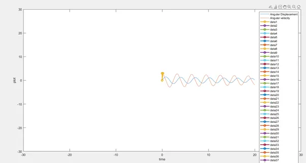
Resolution: I have tried multiple times by trail and error to correct the code. Finally, I have referred to some posts and tried to correct my mistake.