Project 1 - Parsing NASA thermodynamic data
AIM:
- MATLAB program to evaluate the thermodynamic data like Specific heat, Enthalpy and Entropy using the NASA thermodynamic data file.
- Plot Cp, S , H for the local temperature range
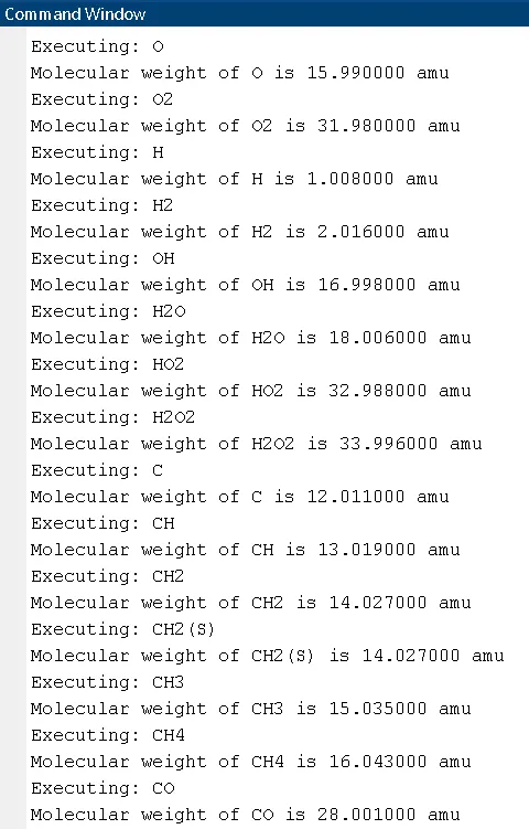
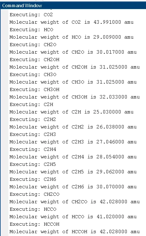
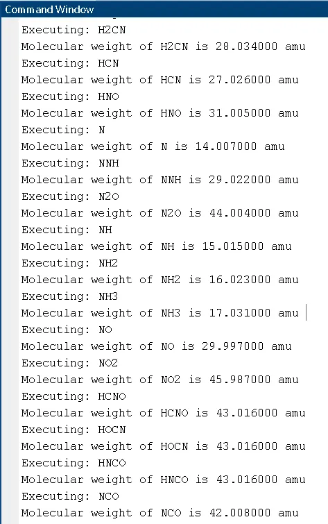
- Calculate molecular weight of the species.
OBJECTIVE:
- Study the thermodynamic properties such as Specific heat, Enthalpy and Entropy for given species.
- File parsing
- Parsing the given data file to read the required data which is needed for calculation of Specific heat, Enthalpy and Entropy.
Ideal gas Thermodynamic properties:
Thermodynamic properties for ideal gases are tabulated in a variety of locations in Chemkin format.
The below format involves two sets of seven constants a1 through a7. These constants are fits to specific heat, enthalpy, and entropy data (or calculations) according to the following formulae:

Specific heat (Cp):
Specific heat is a ratio of the quantity of heat required to raise the temperature of a body one degree to that required to raise the temperature of an equal mass of water one degree.
Units: J/Kg K
Enthalpy (H):
The enthalpy of a thermodynamic system is defined as the sum of its internal energy and the work required to achieve its pressure and volume. Units: J
Entropy(S):
Entropy is a measure of degree of dis-orderness of the system. Units: J/K
R - Universal gas constant : 8.314 J/K-mol
File parsing:
Parsing a file means reading the data from a file. This data can be used in programming.
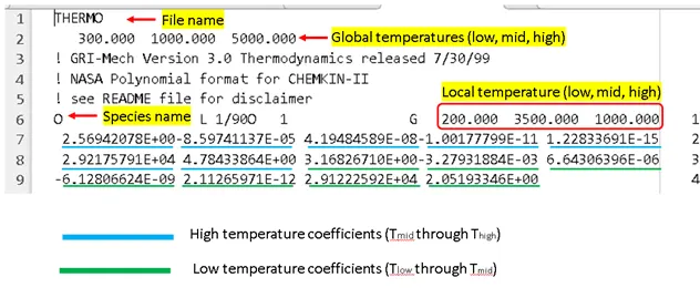
In this case, we have a file where there is thermodynamic data for 53 species. The data can be read as shown in the below image. By using the MATLAB code, the given data needs to be served as input and by using the formulae the Cp, H and S values for different species are calculated.
Function code:
function[Cp H S] = Cp_H_S(a1,a2,a3,a4,a5,a6,a7,R,T)

Cp = (a1 + a2.*T + a3.*T.^2 + a4*T.^3 + a5.*T.^4).*R;
H = (a1 + (a2.*T)./2 + (a3.*T.^2)./3 + (a4.*T.^3)./4 + (a5.*T.^4)./5 + (a6./T)).*R.*T;
S = (a1.*log(T) + a2.*T + (a3.*T.^2)./2 + (a4.*T.^3)./3 + (a5.*T.^4)./4 + a7).*R;

end
Main code:
% Parsing NASA thermodynamic data and calculating Specific heat(Cp),
% Enthalpy(H) and Entropry(S)
clear all
close all
clc

% INPUTS
% value of universal gas constant
R = 8.314;

%% Open the data file and reading it
file_Id = fopen('THERMO.dat', 'r');
% Reading till 2nd line of the file
for i = 1:2
L1 = fgetl(file_Id);
end

%Splitting the line and retrieving the values of global temperatures
Global_temp_line = strsplit(L1, '  ');
Global_temp_low = str2double(Global_temp_line{2});
Global_temp_mid = str2double(Global_temp_line{3});
Global_temp_high = str2double(Global_temp_line{4});

%% Reading the lines till just before the start of species line
for i = 1:3
L2 = fgetl(file_Id);
end

%% Calculating the Cp, H and S. Plot them with respect to local temperatures.
% Here on the species name, temperatures and coefficients  will be retrived and stored.

for i = 1:53
    L3 = fgetl(file_Id);
A = strsplit(L3, '  ');
    Species = A(1);   % Reading 1st cell(Species name) of the splitted line
Species = char(Species); % changing from cell to character

%LOCAL TEMPEARTURE RANGES
T_low_local = str2double(A{end-3});
T_mid_local = str2double(A{end-1});
T_high_local = str2double(A{end-2});

%By fscanf command the floating values will be retrived. fscanf searches for the floating number till
% it finds any other format and stop there. Then it returns the list of
% floating numbers to variable. Here in our case the other format is
% character (Species name).

B = fscanf(file_Id,'%f',[1,218]);

% storing coefficients from each species
a1_high_temp = B(1);
a2_high_temp = B(2);
a3_high_temp = B(3);
a4_high_temp = B(4);
a5_high_temp = B(5);
a6_high_temp = B(7);
a7_high_temp = B(8);

a1_low_temp = B(9);
a2_low_temp = B(10);
a3_low_temp = B(11);
a4_low_temp = B(13);
a5_low_temp = B(14);
a6_low_temp = B(15);
a7_low_temp = B(16);

% range of local temperature
local_temp = T_low_local:T_high_local;

% Calculating Cp,H,S using the defined function
for j = 1:length(local_temp)
    if local_temp < T_mid_local
     [Cp, H, S] =  Cp_H_S(a1_low_temp,a2_low_temp,a3_low_temp,a4_low_temp,a5_low_temp,a6_low_temp,a7_low_temp,R,local_temp);
    else
     [Cp, H, S] =  Cp_H_S(a1_high_temp,a2_high_temp,a3_high_temp,a4_high_temp,a5_high_temp,a6_high_temp,a7_high_temp,R,local_temp);
    end
end

%% Create Plots

figure(i)
t = tiledlayout(3,1,'TileSpacing','Compact');
% subplot(3,1,1)
nexttile
plot(local_temp, Cp,'linewidth',1,'Color','r')
ylabel('Specific heat (J/Kg K')
grid on

% subplot(3,1,2)
nexttile
plot(local_temp, H,'linewidth',1,'Color','g')
ylabel('Enthalpy (J)')
grid on

% subplot(3,1,3)
nexttile
plot(local_temp, S,'linewidth',1,'Color','g')
ylabel('Entropy (J/K)')
grid on

% Main title for the plots
title(t, sprintf('Thermodynamic properties of %s', Species));
xlabel(t,'Local temperature (K)')

fprintf('Executing: %s \n', Species) % To understand which species is executed

% Create a folder in existing folder path
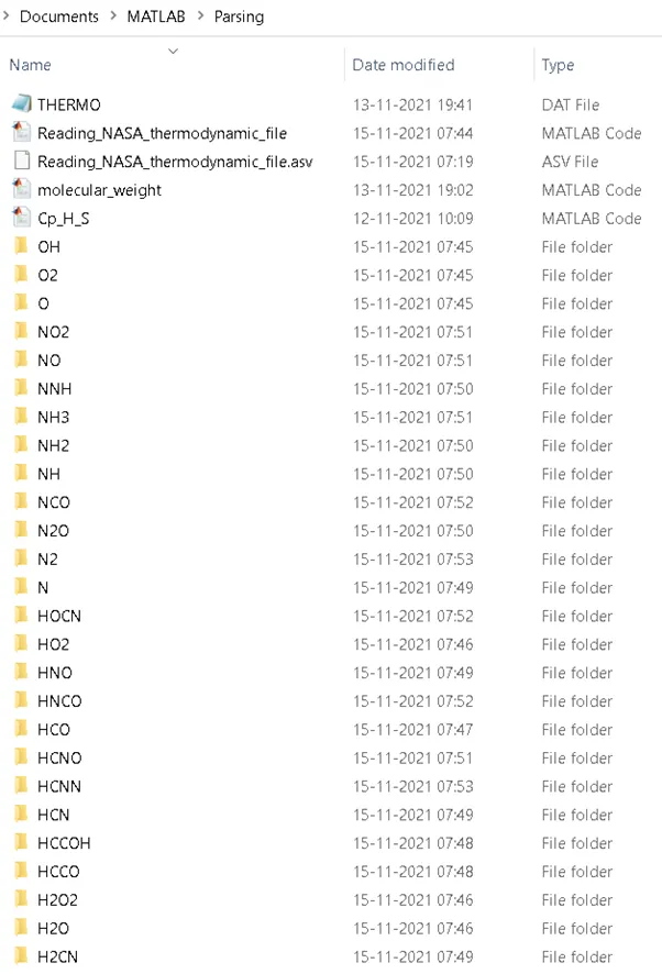
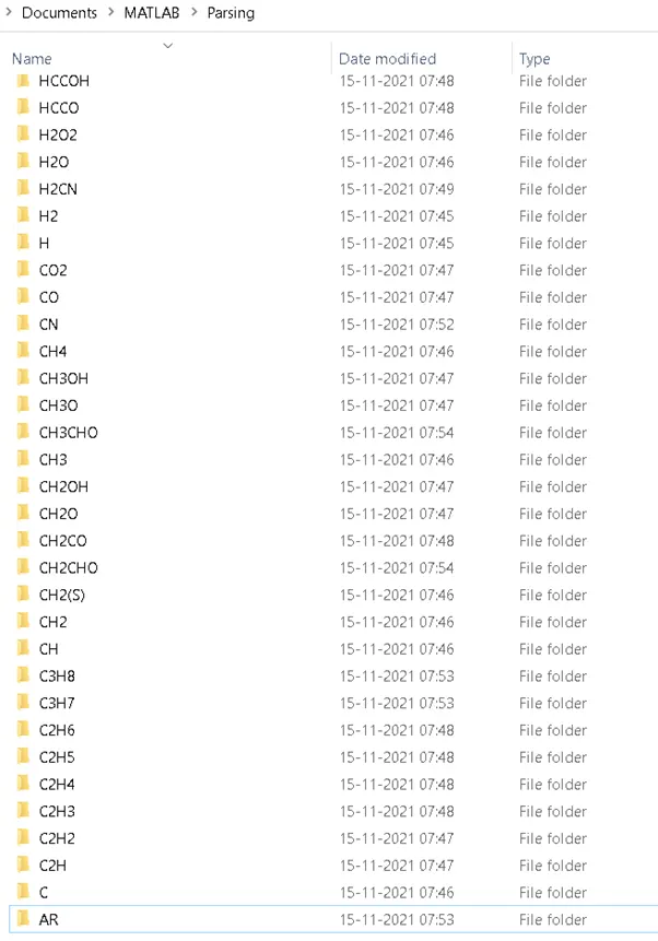
mkdir(['C:\Users\Admin\Documents\MATLAB\Parsing\',Species]);

% Change directory : Go to the created folder
cd(['C:\Users\Admin\Documents\MATLAB\Parsing\',Species]);

% Saving plots
saveas(i, sprintf('Thermodynamic_data_plot_%s .png', Species))

% Come back to the folder where the function file is located, so that it is
% used for next set of loops
cd(['C:\Users\Admin\Documents\MATLAB\Parsing']);

%% Molecular weight of the species

% Defining elements. AR is considered as A because, MATLAB is considering
% 'AR' as two characters, hence there will be mismatch between elements qty
% and atomic weight qty.
elements = ['O','H','C','N','A'];
atomic_weight = [15.99,1.008,12.011,14.007,39.948]; % Defining their atomic weights

molecular_weight = 0;
for i = 1:length(Species)  % this will run the length of species name(characters)
    for j = 1:length(elements)
        if strcmpi(Species(i),elements(j))   % Comparing the letters of species name with each element
            molecular_weight = molecular_weight + atomic_weight(j); % summing the weights
            position = j;
        end
    end
    m = str2num(Species(i)); % if the species name has a number(example: H2) in it, this command will convert from char to number
    if m>1                  % if the number is greater than 1 the below loop is executed else no.
    molecular_weight = molecular_weight + atomic_weight(position)*(m-1);
    end
end
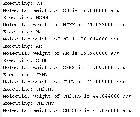
fprintf('Molecular weight of %s is %f amu \n',Species,molecular_weight)  % Printing the weight of each species

end
fclose(file_Id) % Closing the file
Explanation of the code:
- Initially, the given file ‘Thermo.dat’ is fetched into the main code using fopen and access it by read mode. Using ‘fgetl’ a line is read. When ‘fgetl’ is used repeatedly, then the it reads the next lines and so on.
- MATLAB considers the data in a particular line as characters even though we have numbers in that line.
- Using ‘strsplit’ command the line is split into group of strings. These strings are stored as ‘cells’. The command ‘str2double’ is then used to convert the ‘cells’ to ‘double’(numbers). In this way, the global temperatures are read and displayed in work space.
- Similarly using the commands ‘strsplit’ and ‘str2double’, the next lines (local temperature and species name) of the data is fetched and stored in the variables.
- By ‘fscanf’ command the floating values will be retrieved. fscanf searches for the floating number till it finds any other format and stop there. Then it returns the list of floating numbers to variable. Here in our case the other format is character (Species name). In this way the 14 coefficients can be extracted from the data file.
- Now we have all the values required to calculate Cp , H and S. A function is created which has the equations to calculate Cp , H and S for the local temperature range.
- Next step is to plot the Cp , H and S vs local temperature range. Using ‘plot’ and ‘titledlayout’ commands the all the three plots are grouped in a single figure with a required title.
- ‘mkdir’ is used to create a folder to save these plotted images. ‘cd’ (change directory) is used to go to that directory and ‘saveas’ command saves the image in respective folder.
- Once a image is saved in particular folder, then ‘cd’ is used to go back to main folder and the loop continues for all the 53 species.
- Other part of our code is related to calculating the molecular weight of the species. By looking into the species names, we can figure out the elements used i.e 'O','H','C','N','A'.The respective atomic weights are stored in the array.
- The molecular weight is then calculated by comparing the elements with the species characters one by one and summing up the molecular weight. If the species name has a number (example: H2) in it, it is converted from char to double(number). Using another ‘if’ loop the molecular weight of species which has a number (example: H2) is calculated. If there is no number in the species name then this ‘if’ loop is skipped.
- Finally, the molecular weight is printed in the command window using ‘fprintf’ command.
- The above code is repeated for the 53 species listed in the given file. The file is closed using ‘fclose’ command.
Output:
Printing molecular weight in command window
Folders:
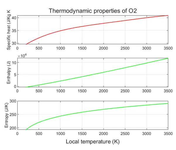
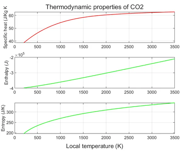
Plots:
Plot for O2
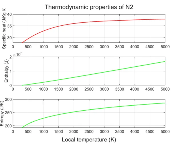
Plot for N2
Plot for CO2
Erros:
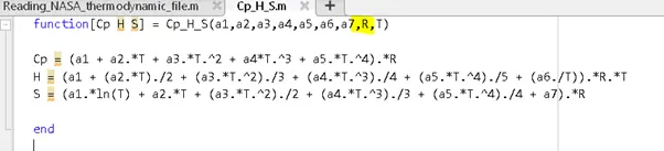
1. Unrecognized varaible 'R"

Corrected by adding it as shown.
2. Unrecognized variable 'ln'

Resolved by changing it to 'log'

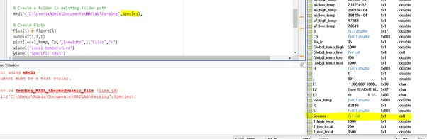
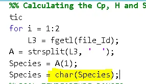
3. The 'Species' variable is in cell format and that is the reason for this error.
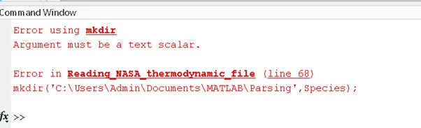
Converted cell to character and resolved it.

References:
https://in.mathworks.com/help/matlab/ref/sscanf.html
https://in.mathworks.com/help/matlab/ref/readlines.html
https://in.mathworks.com/help/matlab/ref/mkdir.html?searchHighlight=mkdir&s_tid=srchtitle_mkdir_1
https://in.mathworks.com/help/matlab/ref/saveas.html?s_tid=doc_ta
https://in.mathworks.com/matlabcentral/answers/174253-how-to-convert-a-1x1-cell-to-a-string
https://in.mathworks.com/help/matlab/ref/tiledlayout.html
https://in.mathworks.com/help/matlab/ref/strcmp.html?s_tid=doc_ta