Week 4.1 - Genetic Algorithm

Try to understand the concept of genetic algorithm by referring to varius sources before you attend this challenge. Look out for information regarding stalagmite function and ways to optimise it.

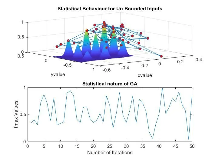
• Write a code in MATLAB to optimise the stalagmite function and find the global maxima of the function.
• Clearly expalin the concept of genetic algorithm in your own words and also explain the syntax for ga in MATLAB in your report.
• Make sure that your code gives the same output, even if it is made to run several times.
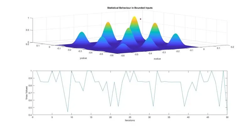
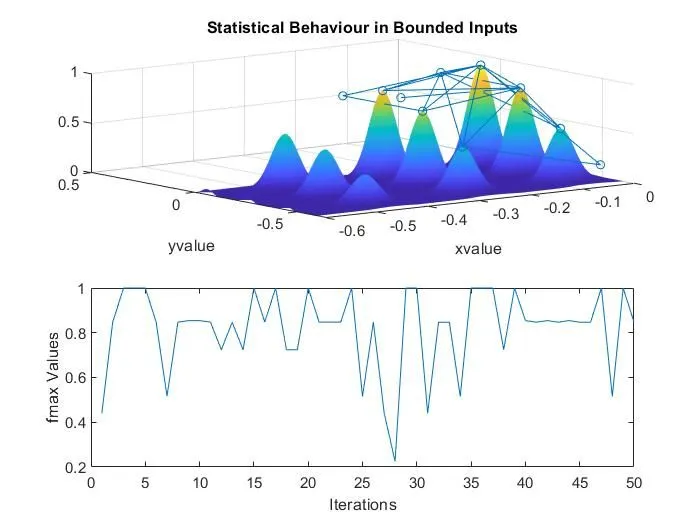
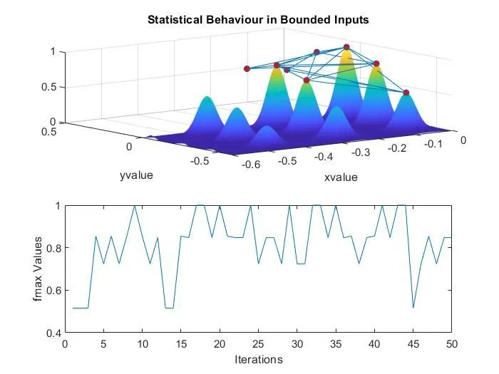
• Plot graphs for all 3 studies and for F maximum vs no. of iterations. Title and axes labels are a must, legends could be shown if necessary.

Concept of GA(Genetic Algorithm)

• The genetic algorithm is a method for solving both constrained and unconstrained optimization problems that are based on the process that drives biological evolution that is natural selection.
• GA follows certain steps in order to produce an optimized result, where ga starts with a selection rule followed by a crossover rule and then a mutation rule.
  • Selection rules select the data points from the data pool and save them as a population, the size of the population can be controlled by the ga syntax.
  • Crossover rules treat the last generation population as parents and create offspring data points from the previous generation and in such a way the population data pool keeps on changing with each iteration.
  • To avoid repetition and induct randomness Mutation rules have been defined which make sure that the population data pool in each iteration is different. The best data or point converges to the optimum value with each iteration.
• It is also necessary to end the algorithm in an efficient manner because after certain iterations the optimum value doesn't vary much.
• The difference between classical derivative-based optimization algorithm and ga is very fundamental
  • GA generates a population of points at each iteration, whereas the classical derivative algorithm generates a single point at each iteration.
  • GA generates a different population for each iteration by using random number generators whereas the Classical derivative algorithm selects the next point in the sequence by a deterministic computation.

The GA solves in certain procedure which is given below

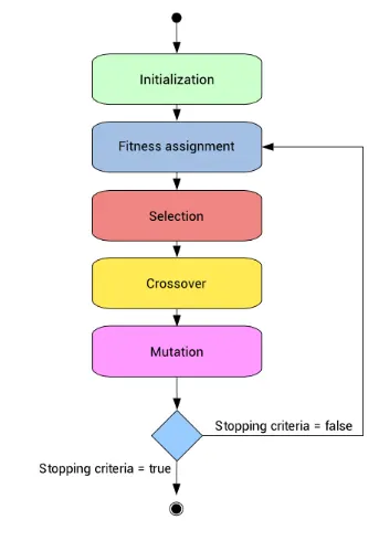
The Genetic algorithm starts with Initialisation followed by fitness assignment then Selection, Crossover, Mutation, Termination respectively.

Syntax for Genetic Algorithm

[inputs,fval] = ga(fun,nvars,A,b,Aeq,beq,lb,ub,nonlcon,options)

2. fun - objective function specified as a function name. In my code @stalagmite_function
3. nvars - Number of variables, specified as a positive integer. In my code 2.
4. A - Linear inequality constraints, specified as a real matrix A is an M by nvars matrix where M is a number of inequalities. For my code, it is [] which means no linear inequality constraints.
5. b - Linear inequality constraints, specified as real vector b is an M-element vector related to the A-matrix. It is a column vector. For my code, it is [] which means no linear inequality constraints.
6. Aeq - Linear equality constraints, specified as a real matrix Aeq is a Me-by-nvars matrix, where Me is the number of equalities. For my code, it is [] which means no linear equality constraints.
7. beq - Linear equality constraints, specifies as a real vector beq is a Me-element vector related to the Aeq matrix. It's a column vector. For my code, it is [] which means no linear equality constraints.
8. lb - Lower bounds, specified as a real vector of doubles. For my code it is [0:0].
9. ub - Upper bounds, specified as a real vector of doubles. For my code, it is [0.5:0.5].
10. nonlcon - Nonlilnear constraints, specified as a function name. nonlcon is a function that accepts a vector x and returns two arrays, c(x) and ceq(x), For my code, it is [] which means nonlinear constraints.
    • c(x) is the array of nonlinear equality constraints at x ga attempts to satisfy `c(x)<=0`
    • ceq(x) is the array of nonlinear equality constraints at x ga attempts to satisfy `ceq(x)=0`
11. options - Optimization options, specified as the output of optimoptions.

Stalagmite function

The function definition of the Stalagmite function is given below

`f_(1,x)=[sin(5.1pix+0.5)]^6`

`f_(1,y)=[sin(5.1piy+0.5)]^6`

`f_(2,x)=exp[-4ln2(x-0.0667)^2/0.64]`

`f_(2,y)=exp[-4ln2(y-0.0667)^2/0.64]`

`f(x,y)=f_(1,x)*f_(2,x)*f_(1,y)*f_(2,y)`

Stalagmite function code

%% Stalagmite function code

function [f]=stalagmite_function(input_vector)

x=input_vector(1);  % First input
y=input_vector(2);  % Second input
 

f1x=(sin(5.2*pi.*x+0.5)).^6;    
f1y=(sin(5.1*pi.*y+0.5)).^6;
f2x=exp(-4*log(2).*(x-0.0667).^2/(0.64));
f2y=exp(-4*log(2).*(y-0.0667).^2/(0.64));
f=-f1x.*f1y.*f2x.*f2y;      % Equation of stalagmite function
end

• The function handle is stalagmite_function
• The input argument is input_vector
• The output of this function will be stored in an array called f.

Code for optimizing Stalagmite function using Genetic algorithm

%% Optimising Stalagmite Function using Genetic Algorithm

clear all
close all
clc

x=linspace(0,0.6,150);      % Creating x-array
y=linspace(0,0.6,150);      % Creating y-array
iterations=50;              % Number of iterations
[xx yy]=meshgrid(x,y);      % Creating a 2D mesh from 1D x,y array

for i=1:length(xx)              % for loop to solve stalagmite function
    for j=1:length(yy)          
        input_vector(1)=xx(i,j);% creating inputs for the function    
        input_vector(2)=yy(i,j);% creating inputs for the function    
        f(i,j)=stalagmite_function(input_vector); % Assigning function value to f(i,j)
    end
end
[input_val,f_val]=ga(@stalagmite_function,2)    % Optimising x and y using genetic algorithm 


%% Analysing statistical behavior of Genetic algorithm for unbound inputs

tic     % Starting the stop watch timer to evaluate elapsed time
for k=1:iterations                          % Creating for loop to make different iteratration of GA optimisation
    [input,fval]=ga(@stalagmite_function,2);% Optimising using GA for unbound inputs
    x1(k)=input(1);     % Saving input(1) in x1 array
    y1(k)=input(2);     % Saving input(2) in y1 array
    f1(k)=fval;         % Saving fval in f1 array
end
toc     % Stoping the stop watch             

%Plots
figure(1)       % Creating new figure window
subplot(2,1,1)  % First subplot 
surf(-xx,-yy,-f)% Surface plot of Stalagmite function
shading interp  % To disable grid lines from surface plot
hold on         % To create another plot in same subplot
plot3(-x1,-y1,-f1,'marker','o','markersize',5,'markerfacecolor','r') % Ploting all the function optimum values in same subplot
title('Statistical Behaviour for Un Bounded Inputs') % Title of first subplot
xlabel('xvalue')
ylabel('yvalue')
hold off
subplot(2,1,2)      % Second subplot
plot(-f1)           % Plotting fmax values for each iterations
title('Statistical nature of GA')   % Title of second subplot
xlabel('Number of Iterations')
ylabel('fmax Values')

%% Analysing statistical behavior of Genetic algorithm for bounded inputs

tic         % Starting the stop watch timer to evaluate elapsed time
for i=1:iterations      % Creating for loop to make different iteratration of GA optimisation
    [input,fval]=ga(@stalagmite_function,2,[],[],[],[],[0:0],[0.5:0.5]);
    x2(i)=input(1);     % Saving input(1) in x3 array
    y2(i)=input(2);     % Saving input(2) in y3 array
    f2(i)=fval;         % Saving fval in f3 array
end
toc         % Stoping the stop watch

% Plots             
figure(2)           % Creating new figure window
subplot(2,1,1)      % First subplot 
surf(-xx,-yy,-f)    % Surface plot of Stalagmite function       
shading interp      % To disable grid lines from surface plot
hold on             % To create another plot in same subplot
plot3(-x2,-y2,-f2,'marker','o','markersize',5,'markerfacecolor','r') % Ploting all the function optimum values in same subplot
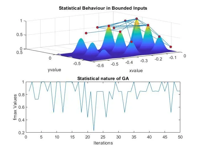
title('Statistical Behaviour in Bounded Inputs')  % Title of first subplot
xlabel('xvalue')
ylabel('yvalue')
subplot(2,1,2)      % Second subplot
plot(-f2)           % Plotting fmax values for each iterations
title('Statistical nature of GA')   % Title of second subplot
xlabel('Iterations')
ylabel('fmax Values')


%% Analysing Genetic algorithm for increase in population size
%Increasing the GA population size
option=optimoptions('ga');
option=optimoptions(option,'PopulationSize',1000);


tic         % Starting the stopwatch timer to evaluate elapsed time
for m=1:iterations
    [input,fval]=ga(@stalagmite_function,2,[],[],[],[],[0:0],[0.5:0.5],[],[],option);
    x3(m)=input(1);     % Saving input(1) in x3 array
    y3(m)=input(2);     % Saving input(2) in y3 array
    f3(m)=fval;         % Saving fval in f3 array
end
toc         % Stoping the stop watch

%Plots
figure(3)           % Creating new figure window
subplot(2,1,1)      % First subplot 
surf(-xx,-yy,-f)    % Surface plot of Stalagmite function
shading interp      % To disable grid lines from surface plot
hold on             % To create another plot in same subplot
plot3(-x3,-y3,-f3,'marker','o','markersize',5,'markerfacecolor','r') % Ploting all the function optimum values in same subplot
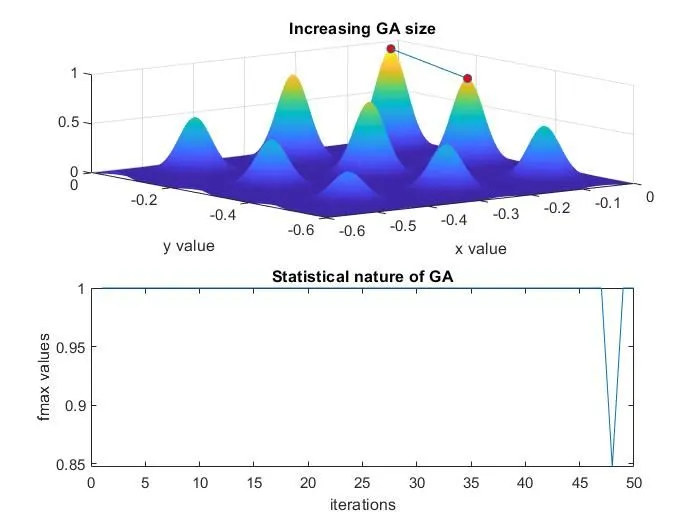
title('Increasing GA size')     % Title of first subplot
xlabel('x value')
ylabel('y value')
subplot(2,1,2)      % Second subplot
plot(-f3)           % Plotting fmax values for each iterations
title('Statistical nature of GA')   % Title of second subplot
xlabel('iterations')
ylabel('fmax values')

Explanation to the Code

• Code is divided into 4 parts
  • 1st part is to plot a stalagmite function using Matlab.
  • 2nd part is to analyze the statistical behavior of the Genetic algorithm for unbounded inputs.
  • 3rd part is to analyze the statistical behavior of the Genetic algorithm for bounded inputs.
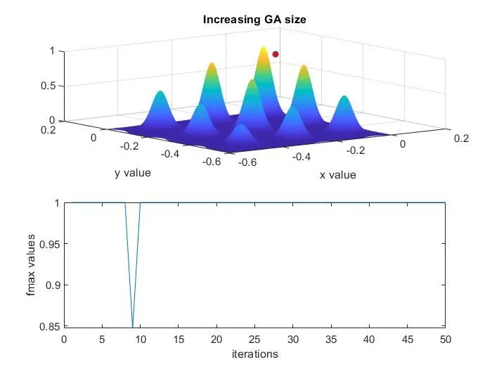
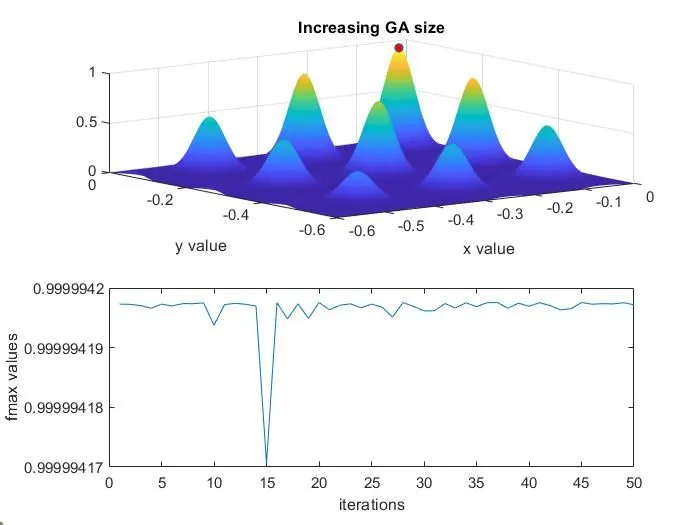
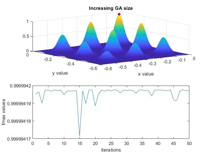
  • 4th part is to analyze the effect of change of population size on the Genetic algorithm solving process.

1st Part

• Code starts with clear all, close all, clc which is used to clear the garbage data from the memory.
• Two equal 1D arrays have been defined in name of x and y respectively.
• A 2D mesh has been created from x and y using syntax meshgrid.
• A for loop has been constituted to calculate stalagmite_function value for each input from meshgrid.

2nd Part

• tic is used to start the stopwatch which calculates the elapsed time to run the loop.
• for loop is constituted to make a number of iterations of ga and store it in arrays respectively.
• Here the input arguments were unbounded so only considered function handle and number of variables to calculate the optimum value of the function.
• Both input and output arguments have been saved in respective arrays.
• Using the saved arrays plots have been made as follows
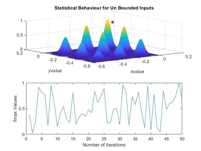
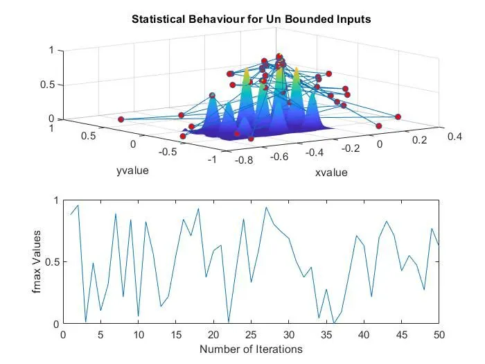
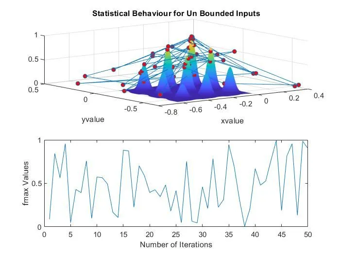
  • In the first figure window, two subplots have been made a surface plot for stalagmite function, different optimum values of function respectively in the first plot and in the second plot, the variation of optimum value with iterations have been given.

3rd Part

• tic is used to start the stopwatch which calculates the elapsed time to run the loop.
• for loop is constituted to make a number of iterations of ga and store it in arrays respectively.
• Here the input arguments were bounded so it is important to consider the bound condition for the optimum calculation.
• Both input and output arguments have been saved in respective arrays.
• Using the saved arrays plots have been made as follows
  • In the first figure window, two subplots have been made a surface plot for stalagmite function, different optimum values of function respectively in the first plot and in the second plot, the variation of optimum value with iterations have been given.

4th Part

• Here a new syntax option and optimoptions have been used to consider the change in PopulationSize to 1000.
• tic is used to start the stopwatch which calculates the elapsed time to run the loop.
• for loop is constituted to make a number of iterations of ga and store it in arrays respectively.
• It is important to consider the option to make it effective in the calculation so a new input argument has to assign, option.
• Both input and output arguments have been saved in respective arrays.
• Using the saved arrays plots have been made as follows
  • In the first figure window, two subplots have been made a surface plot for stalagmite function, different optimum values of function respectively in the first plot and in the second plot, the variation of optimum value with iterations have been given.

Results

Figure(1)

• Run1
  • 
• This plot is to show the unbounded optimum for one iteration of ga.
• Run2
  • 
• Run3
  
  • 
• Run4
  • 

Figure(2)

• Run1
  • 
• Run2
  • 
• Run3
  • 
• Run4
  • 

Figure(3)

• Run1
  • 2Run1
• Run2
  • 
• Run3
  • 
• Run4
  • 

Conclusion

From the above study, I've understood the optimization of the stalagmite function using a genetic algorithm.

The different use case scenario of ga and their statistical behavior is analyzed.

Errors

• 
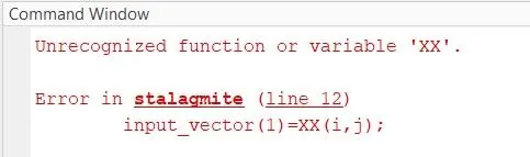
  • Here the error was a different argument is used for xx

• 
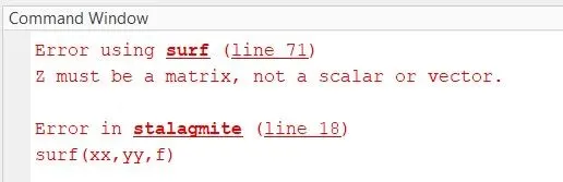
  • Due wrong function code the f became a scalar instead of an array.
• 
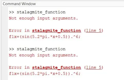
  • Treated inputs as a scalar and assigned two values which printed this error.

..........................................................................................................................end..........................................................................................................