Week 4.1 - Genetic Algorithm

Brief On Genetic Algorithm

Genetic algorithm is an optimization technique used to solve non linear and non differential problems that is based on natural selection.The genetic algorithm repeatedly modifies the individual solutions.At each step, the genetic algorithm selects individuals at random from the current population to be parents and uses them to produce the children for the next generation.

The most important phases of genetic algorithm are as follows:

1)Initial population

2)Fitness Function(fitness score)

3)Selection(i.e adult transformation)

4)Crossover

5)Mutation

The steps GA(Genetic algorithm) works on in matlab is as follows:

• GA's works with the coding of genetic parameters set.
• GA's search from a population of points.
• GA's use objective function information.
• GA's use probabilistic transition rules.

Program to Optimize the Stalagmite Function and to find Global maxima

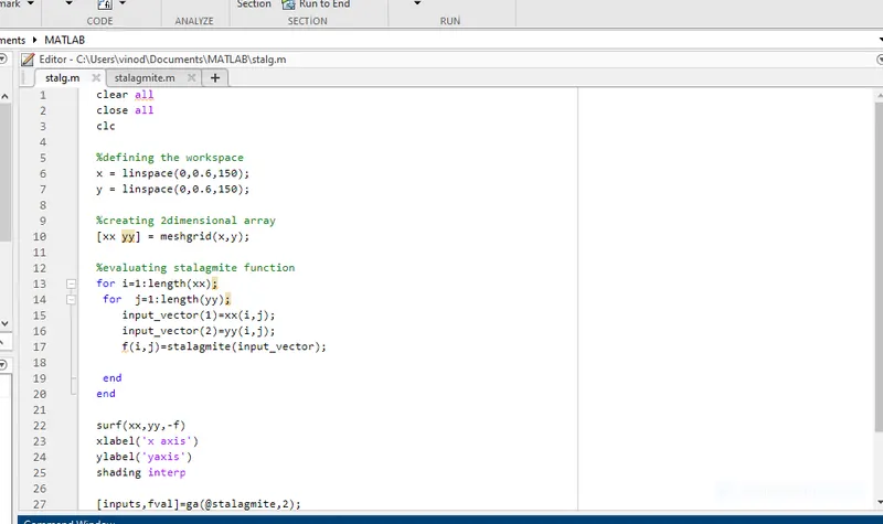
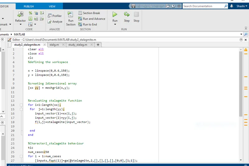
In this picture the x and y arrays has been introduced with the linspace command between the range of 0 and 0.6 for 150 values.Then a 2dimensional array has been asssigned with the tag xx and yy by using meshgrid command.For evaluating stalagmite function, 2 for loops loop has been constructed for both xx and yy seperately.A stalagmite function has been defined and the code of that will be posted below.Then the surf command is used to plot the xx and yy along with -ve values of f values which gives us the global maxima.

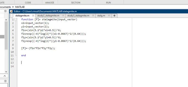
In this picture, a stalagmite function has been defined for the given function f(x,y)=f1x*f2x*f1y*f2y.

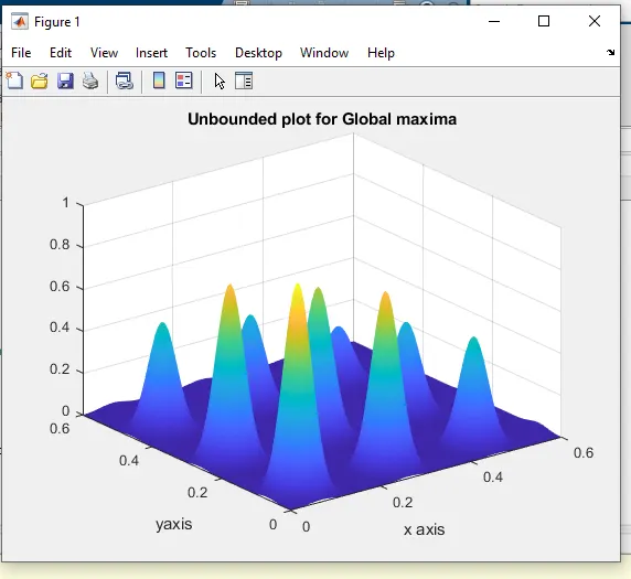
The plot for global maxima with an unbounded inputs is as follows:

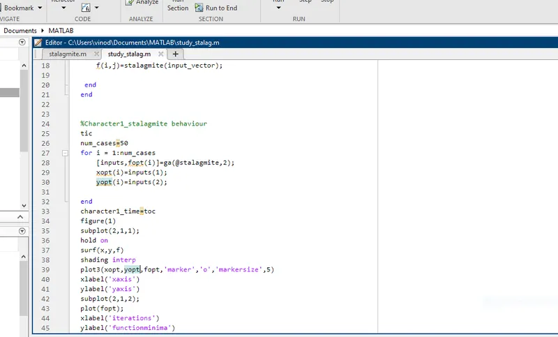
In the below picture,as we seen earlier we have got the global maxima value for the unbounded figure and without iterations,so here we have run through 50 iterations by usind the num_cases syntax for each variable so to get the best results in the way of finding the optimize point which may be good enough.So here a for loop ahs been constructed for the new variables x(opt) and y(opt).Then the command figure(1) is used to get a new figure window and subpolt is assugnet to plot 2 plots in a same window for the obtain x(opt),y(opt) and f(opt)values.

an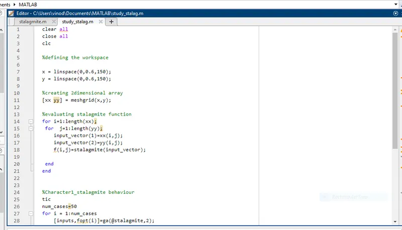

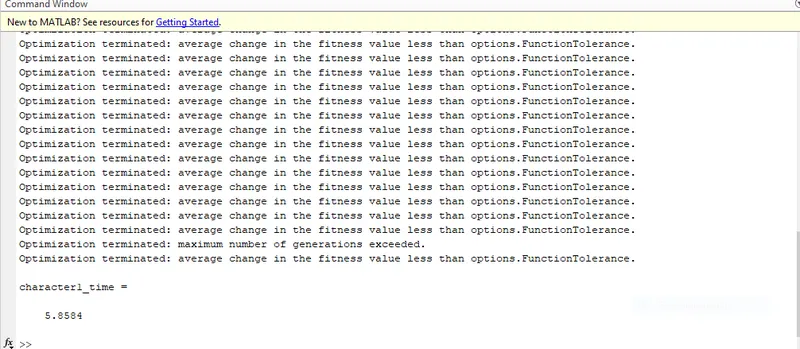
The output over the study 1 of a stalagmite function and the time taken to complete the optimization will be shown below:

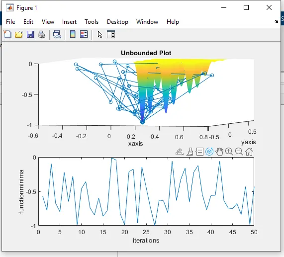
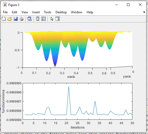
The plot between function minima and no of iterations is as follows

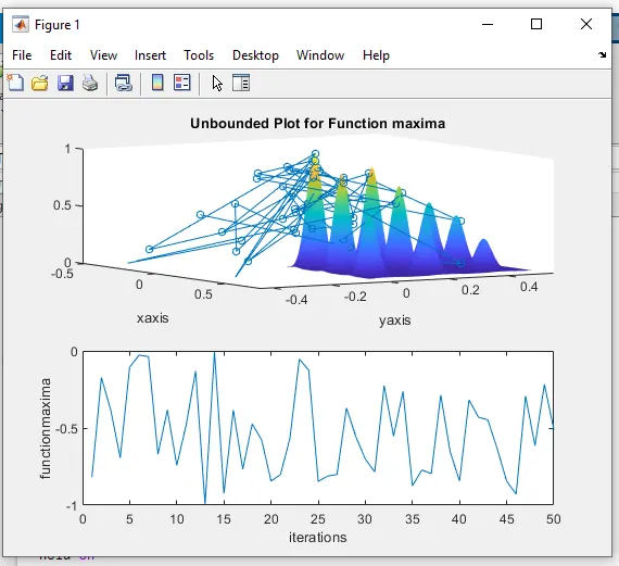
The plot between function maxima vs iterations is as follows,where the -ve sign will be used while defining the stalagmite function to get the maxima value and even while plotting the -ve sign for f(opt) values to get the same.

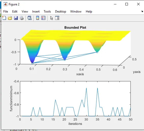
So as we seen above we have tried with the n number iterations to optimize the function,from that we understood the x and y values could go behind or above the given range i.e between 0 and 0.6.So an upper and lower bound which will be in the range of (0,0) and (1,1) has to be defined to get a precised optimise value and the syntax of ga is assigned with the fucntion handle,nvars(i.e number of variables which will be 2 in this case) and the upper and lower bound as shown below:

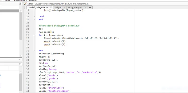
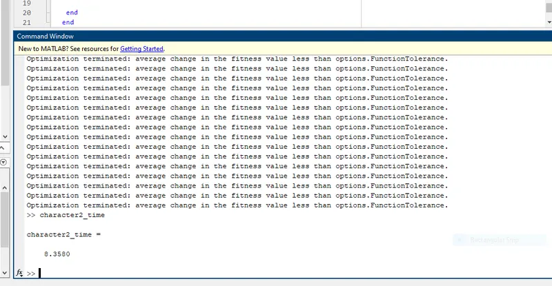
For the given upper and lower bounds as earlier defined and to calculate the time taken we have used tic and toc command, the advantage of that will be shown below in the output.

The plot between functionminima and iteration is shown below:

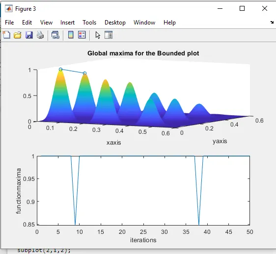
The plot for functionmaxima and iterations is shown below:

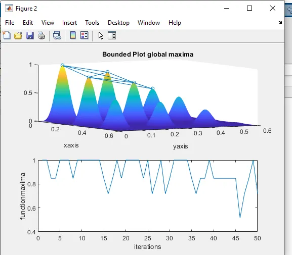
So as we seen in the above study,we have good a better solution for optimization but to get the precise and best result, the only thing need to be done is by reducing the workspace or by increasing the size of initial population.That has been done in the bleow program.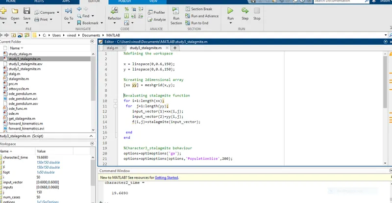

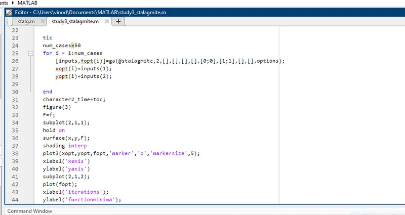
As you can see above the population size has been defined to 200 along with the upper and lower bounds.Even the syntax of ga has been assigned eith the tag options which has defined above as the population size.So in next figure you can look at the plot and understand how precise solution we have got by decresing the workspace just by giving more initial individual values.Before the plot the output and the time taken in this study will be shown below:

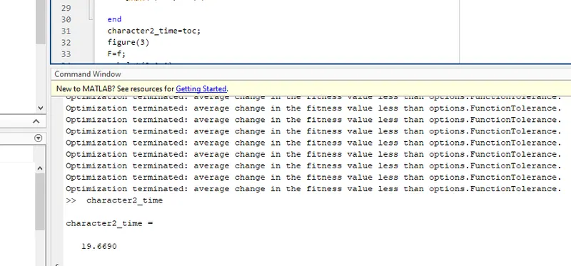
The plot between functionminima and the iterations in this study is as follows:

The plot for functionmaxima vs iterations for this study will be obtained by using the -ve sign while calling the function and plotting:

The code sample for all the studies has pasted below:

clear all
close all
clc

%defining the workspace
x = linspace(0,0.6,150);
y = linspace(0,0.6,150);

%creating 2dimensional array
[xx yy] = meshgrid(x,y);

%evaluating stalagmite function
for i=1:length(xx);
 for  j=1:length(yy);
    input_vector(1)=xx(i,j);
    input_vector(2)=yy(i,j);
    f(i,j)=stalagmite(input_vector);

 end
end

surf(xx,yy,-f)
xlabel('x axis')
ylabel('yaxis')
shading interp

[inputs,fval]=ga(@stalagmite,2);



%stalagmite function
function [f]= stalagmite(input_vector)
x1=input_vector(1);
y1=input_vector(2);
f1x=(sin(5.1*pi*x1+0.5))^6;
f2x=exp((-4)*log(2)*((x1-0.0667)^2/(0.64)));
f1y=(sin(5.1*pi*y1+0.5))^6;
f2y=exp((-4)*log(2)*((y1-0.0667)^2/(0.64)));

[f]=-(f1x*f2x*f1y*f2y);

end


%Character1_stalagmite behaviour
tic
num_cases=50
for i = 1:num_cases
    [inputs,fopt(i)]=ga(@stalagmite,2);
    xopt(i)=inputs(1);
    yopt(i)=inputs(2);

end
character1_time=toc
figure(1)
subplot(2,1,1);
F=-f
hold on
surf(x,y,F)
shading interp
plot3(xopt,yopt,-fopt,'marker','o','markersize',5)
xlabel('xaxis')
ylabel('yaxis')
subplot(2,1,2);
plot(fopt);
xlabel('iterations')
ylabel('functionmaxima')

%Character2_stalagmite behaviour
tic
num_cases=50
for i = 1:num_cases
    [inputs,fopt(i)]=ga(@stalagmite,2,[],[],[],[],[0;0],[1;1]);
    xopt(i)=inputs(1);
    yopt(i)=inputs(2);

end
character2_time=toc;
F=-f;
figure(2)
subplot(2,1,1);
hold on
surface(x,y,F)
shading interp
plot3(xopt,yopt,-fopt,'marker','o','markersize',5)
xlabel('xaxis')
ylabel('yaxis')
subplot(2,1,2);
plot(-fopt);
xlabel('iterations')
ylabel('functionmaxima')

%Character3_stalagmite behaviour
options=optimoptions('ga');
options=optimoptions(options,'PopulationSize',200);

tic
num_cases=50
for i = 1:num_cases
    [inputs,fopt(i)]=ga(@stalagmite,2,[],[],[],[],[0;0],[1;1],[],[],options);
    xopt(i)=inputs(1);
    yopt(i)=inputs(2);

end
character3_time=toc;
figure(3)
F=-f;
subplot(2,1,1);
hold on
surface(x,y,F);
shading interp
plot3(xopt,yopt,-fopt,'marker','o','markersize',5);
xlabel('xaxis')
ylabel('yaxis')
subplot(2,1,2);
plot(-fopt);
xlabel('iterations');
ylabel('functionmaxima');