Week 4.1 - Genetic Algorithm

AIM:

• Optimise the stalagmite function.
• Plot graphs for all 3 studies and for F maximum vs no. of iterations.

PROCEDURE:

clear all
close all
clc

% Generating the grid space where we need to calculate the value of stalagmite function

x=linspace(0,0.6,150);
y=linspace(0,0.6,150);
[XX,YY]=meshgrid(x,y);
    
num_cases=50;       %Number of itreations we are running to get optimised values


% generating the surface plot for the stalagmite function using surfc

for i=1:length(XX)
     for j=1:length(YY)
             input_vector(1)=XX(i,j);
             input_vector(2)=YY(i,j);
             f(i,j)=stalagmite(input_vector);   %values of function is generated in given search space
     end
 end
 
surfc(XX,YY,-f);       %generating the surface plot
shading interp      %To remove the lines produced by the mesh grid
       
        
       
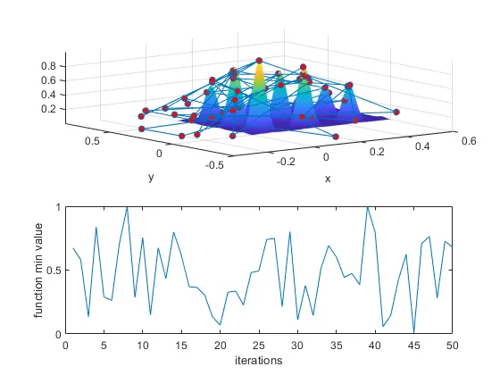
% behaviour of ga function in predicted optimised values       
% without upper and lower bounds
        
tic                             %calculating the time take for iterations through tic and toc command
for i=1:num_cases
    
    [inputs,fopt(i)]=ga(@stalagmite,2);     %ga will sent the optimised values of stalagmite
    xopt(i)=inputs(1);                      %at each iteration
    yopt(i)=inputs(2);
    
end
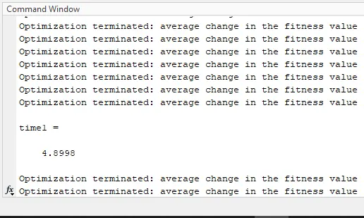
time1=toc                  %time taken for the iteration is calculated using tic toc function
    
% Plotting the surface plot
figure(1)

subplot(2,1,1)

surfc(XX,YY,-f);      
hold on
shading interp
plot3(xopt,yopt,-fopt,'marker','o','markersize',5,'markerfacecolor','r'); %data points will be marked in a 3D space
xlabel('x');
ylabel('y');
grid on

subplot(2,1,2)
plot(-fopt);
xlabel('iterations')
ylabel('function min value')
        
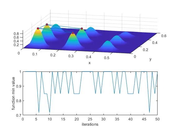
% Defining the upper and lower bounds for better optimised values

tic                                %calculating the study taken t
for j=1:num_cases
    
    [inputs,fopt(j)]=ga(@stalagmite,2,[],[],[],[],[0;0],[0.6;0.6]);   %ga sends the optimized value of the stalagmite function      
    xopt(j)=inputs(1);                                            %for each iteration
    yopt(j)=inputs(2);
    
end
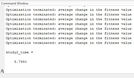
study2_time=toc
    
%Plotting the generated optimised value for second type of optimisation
figure(2)
    
subplot(2,1,1)
hold on
surfc(XX,YY,-f)
shading interp
plot3(xopt,yopt,-fopt,'marker','o','markersize',5,'markerfacecolor','r');
xlabel('x');
ylabel('y');
grid on
subplot(2,1,2)
plot(-fopt);
xlabel('iterations')
ylabel('function min value')
 
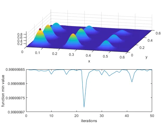
% Population size is changed using optimoptions function
 
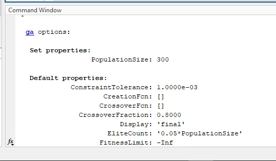
 options=optimoptions('ga','populationsize',300)        %increaing the size of a parameter called population by using
                                                        %optimoptions function
 
 tic                                                    
for k=1:num_cases
    
    [inputs,fopt(k)]=ga(@stalagmite,2,[],[],[],[],[0;0],[0.6;0.6],[],[],options);
     xopt(k)=inputs(1);
     yopt(k)=inputs(2);         
     
end
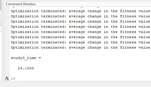
study3_time=toc
    
%plotting the third set of optimised values
figure(3)
    
subplot(2,1,1)  %first subplot
hold on
surfc(XX,YY,-f)
shading interp
plot3(xopt,yopt,-fopt,'marker','o','markersize',5,'markerfacecolor','r');
xlabel('x');
ylabel('y');
grid on
subplot(2,1,2)  %second subplot
plot(-fopt);
xlabel('iterations')
ylabel('function min value')

RESULTS: