Project 2 - Rankine cycle Simulator

AIM:

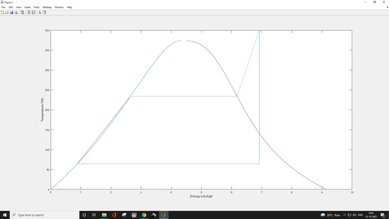
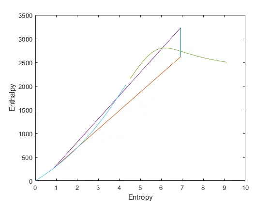
Write a matlab code to simulate Rankine cycle and plot Enthalpy vs entropy chart, Temperature vs Entropy chart, calculate the net work done and efficiency of the cycle.

PROCEDURE:

clear all
close all
clc

sprintf("\n   RANKINE CYCLE SIMULATOR    \n");
sprintf("\n 1-2 Isentropic expansion");
sprintf("\n 2-3 Constant pressure heat rejection at condenser");
sprintf("\n 3-4 Isentropic compression in pump");
sprintf("\n 4-1 Constant pressure heat addition at boiler");

%user inputs for turbine pressure and temperature
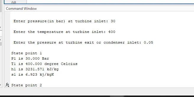
p1=input("\n Enter pressure(in bar) at turbine inlet: ");
t1=input("\n Enter the temperature at turbine inlet: ");
p2=input("\n Enter the pressure at turbine exit or condenser inlet: ");



%state point 1
%water leaves boiler as superheated steam and enters turbine
fprintf('\nState point 1\n')
p1;  %input value
t1;  %input value
h1= XSteam('h_pT',p1,t1);
s1= XSteam('s_pT',p1,t1);

fprintf('P1 is %3.3f Bar\n',p1);
fprintf('T1 is %3.3f degree Celcius\n',t1);

fprintf('h1 is %3.3f kJ/kg\n',h1);
fprintf('s1 is %3.3f kj/kgK\n',s1);


%state point 2
%Leaves turbine and enters condenser
fprintf('\nState point 2\n')
p2;
s2=s1;
power=(1-(1/1.4));
t2=t1*((p2/p1)^power);
h2=XSteam('h_pT',p2,t2);
w_turbine=h1-h2;

%displaying in command window
fprintf('P2 is %3.3f Bar\n',p2);
fprintf('T2 is %3.3f degree Celcius\n',t2);

fprintf('h2 is %3.3f kJ/kg\n',h2);
fprintf('s2 is %3.3f kj/kgK\n',s2);


%State point 3
%water enters pump as saturated liquid

p3=p2;
t3=t2; %constant temperature and pressure heat rejection at condenser


h3=XSteam('hL_T',t3);

v3=XSteam('vL_p',p3);
s3=XSteam('sL_t',t3);   %sf1

%displaying in command window
fprintf('\nState point 3\n')
fprintf('P3 is %3.3f Bar\n',p3);
fprintf('T3 is %3.3f degree Celcius\n',t3);

fprintf('h3 is %3.3f kJ/kg\n',h3);
fprintf('s3 is %3.3f kj/kgK\n',s3);

%state point 4
%water enters boiler as compressed liquid
fprintf('\nState point 4\n')
p4=p1;
s4=s3; 
h4=XSteam('h_ps',p4,s4);
t4 = XSteam('T_hs',h4,s4);

h41 = XSteam('hL_p',p4);
s41 = XSteam('sL_p',p4);
h42 = XSteam('hV_p',p4);
s42 = XSteam('sV_p',p4);
t41 = XSteam('T_hs',h41,s41);
t42 = XSteam('T_hs',h42,s42);


%displaying in command window
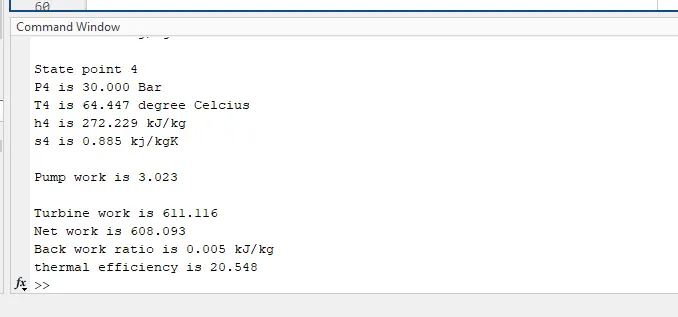
fprintf('P4 is %3.3f Bar\n',p4);
fprintf('T4 is %3.3f degree Celcius\n',t4);

fprintf('h4 is %3.3f kJ/kg\n',h4);
fprintf('s4 is %3.3f kj/kgK\n',s4);

%work input, work output, efficiency calculation
w_pump=h4-h3;
fprintf('\nPump work is %3.3f \n',w_pump);
fprintf('\nTurbine work is %3.3f \n',w_turbine);

w_net=w_turbine-w_pump;
fprintf('Net work is %3.3f \n',w_net);

backworkratio=w_pump/w_turbine;
fprintf('Back work ratio is %3.3f kJ/kg\n',backworkratio);

qin=h1-h4; %heat input
thermalefficiency=(w_net/qin)*100;
fprintf('thermal efficiency is %3.3f \n',thermalefficiency);

%Calculating the Entropy and Enthapy at the saturation curve at:

temperature = linspace(0,500,500);

for i = 1:length(temperature)

sv(i) = XSteam('sV_T',temperature(i));
sl(i) = XSteam('sL_T',temperature(i));

hv(i) = XSteam('hV_T', temperature(i));
hl(i) = XSteam('hL_T', temperature(i));

end

%plotting Temperature vs entropy plot
figure(1)
plot([s1 s2],[t1 t2],[s2 s3],[t2 t3],[s3 s4],[t3 t4],[s4 s41],[t4 t41],[s41 s42],[t41 t42],[s42 s1],[t42 t1])
hold on
plot(sv,temperature) %saturated vapour line
plot(sl,temperature)  %saturated liquid line
xlabel('Entropy');
ylabel('Temperature');

%plotting enthalpy vs entropy
figure(2)
plot([s1 s2],[h1 h2],[s2 s3],[h2 h3],[s3 s4],[h3 h4],[s4 s1],[h4 h1])
hold on
plot (sv,hv)  
plot (sl,hl)
xlabel('Entropy');
ylabel('Enthalpy');

RESULTS: