Week 4.1 - Genetic Algorithm

Aim:- Write a code in MATLAB to optimise the stalagmite function and find the global maxima of the function.

Objectives:-

• Expalin the concept of genetic algorithm in your own words and explain the syntax for ga in Matlab.
• Plot graphs for all 3 studies and for F maximum vs no. of iterations

Concept of Genetic Algorithm:-(Referance from https://www.tutorialspoint.com/genetic_algorithms/genetic_algorithms_introduction.htm)

Optimmization:-

Optimization is the process of making something better. In any process, we have a set of inputs and a set of outputs

Optimization refers to finding the values of inputs in such a way that we get the “best” output values. The definition of “best” varies from problem to problem, but in mathematical terms, it refers to maximizing or minimizing one or more objective functions, by varying the input parameters.

The set of all possible solutions or values which the inputs can take make up the search space. In this search space, lies a point or a set of points which gives the optimal solution. The aim of optimization is to find that point or set of points in the search space

Genetic Algorithm:-

Nature has always been a great source of inspiration to all mankind. Genetic Algorithms (GAs) are search based algorithms based on the concepts of natural selection and genetics. GAs are a subset of a much larger branch of computation known as Evolutionary Computation.

GAs were developed by John Holland and his students and colleagues at the University of Michigan, most notably David E. Goldberg and has since been tried on various optimization problems with a high degree of success.

In GAs, we have a pool or a population of possible solutions to the given problem. These solutions then undergo recombination and mutation (like in natural genetics), producing new children, and the process is repeated over various generations. Each individual (or candidate solution) is assigned a fitness value (based on its objective function value) and the fitter individuals are given a higher chance to mate and yield more “fitter” individuals. This is in line with the Darwinian Theory of “Survival of the Fittest”.

In this way we keep “evolving” better individuals or solutions over generations, till we reach a stopping criterion.

Genetic Algorithms are sufficiently randomized in nature, but they perform much better than random local search (in which we just try various random solutions, keeping track of the best so far), as they exploit historical information as well.

Advantagges of GAs:-

GAs have various advantages which have made them immensely popular. These include −

• Does not require any derivative information (which may not be available for many real-world problems).

• Is faster and more efficient as compared to the traditional methods.

• Has very good parallel capabilities.

• Optimizes both continuous and discrete functions and also multi-objective problems.

• Provides a list of “good” solutions and not just a single solution.

• Always gets an answer to the problem, which gets better over the time.

• Useful when the search space is very large and there are a large number of parameters involved.

Limitation of GAs:-

Like any technique, GAs also suffer from a few limitations. These include −

• GAs are not suited for all problems, especially problems which are simple and for which derivative information is available.

• Fitness value is calculated repeatedly which might be computationally expensive for some problems.

• Being stochastic, there are no guarantees on the optimality or the quality of the solution.

• If not implemented properly, the GA may not converge to the optimal solution.

GA - Motivation:-

Genetic Algorithms have the ability to deliver a “good-enough” solution “fast-enough”. This makes genetic algorithms attractive for use in solving optimization problems. The reasons why GAs are needed are as follows.

Solving Difficult Problems:-

In computer science, there is a large set of problems, which are NP-Hard. What this essentially means is that, even the most powerful computing systems take a very long time (even years!) to solve that problem. In such a scenario, GAs prove to be an efficient tool to provide usable near-optimal solutions in a short amount of time.

Failure of Gradient Based Methods:-

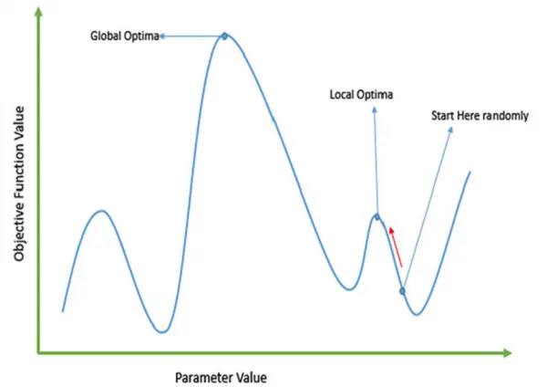
Traditional calculus based methods work by starting at a random point and by moving in the direction of the gradient, till we reach the top of the hill. This technique is efficient and works very well for single-peaked objective functions like the cost function in linear regression. But, in most real-world situations, we have a very complex problem called as landscapes, which are made of many peaks and many valleys, which causes such methods to fail, as they suffer from an inherent tendency of getting stuck at the local optima as shown in the following figure.

Getting a Good Solution Fast:-

Some difficult problems like the Travelling Salesperson Problem (TSP), have real-world applications like path finding and VLSI Design. Now imagine that you are using your GPS Navigation system, and it takes a few minutes (or even a few hours) to compute the “optimal” path from the source to destination. Delay in such real world applications is not acceptable and therefore a “good-enough” solution, which is delivered “fast” is what is required.

Governing Equation:-

`f(x,y) = funderset(1,x) * funderset(2,x)* funderset(1,y) *funderset(2,y)`

`funderset(1,x)= [sin(5.1pix+0.5)]^6`

`funderset(1,y)= [sin(5.1pix+0.5)]^6`

`funderset(2,x)= [-4In(2)*{(x-0.0667)^2}/{0.64}]`

`funderset(2,y)= [-4In(2)*{(x-0.0667)^2}/{0.64}]`

Body of the Content:-

Program in Matlab:-

%function [f] = stalagmite(input_vector)

function [f] = stalagmite(input_vector)

x = input_vector(1);
y = input_vector(2);

f1 = (sin(5.1*pi*x+0.5))^6;
f2 = (sin(5.1*pi*y+0.5))^6;
f3 = exp(-4*log(2)*(x-0.0667)^2/0.64);
f4 = exp(-4*log(2)*(y-0.0667)^2/0.64);

f = -(f1*f2*f3*f4);
end

Code Explanation:-

1.This function defines the stalagmite function to be used in main function.

2.The input vactors x and y will be asigned with the required values in the main function.

Main Code:-

clear all
close all
clc

%defining our search space
x = linspace(0,0.6,150);
y = linspace(0,0.6,150);
num_cases = 50
[xx yy] = meshgrid(x,y);

%Evaluating the stalagmite function
for i = 1:length(xx)
for j = 1:length(yy)
input_vector(1) = xx(i,j);
input_vector(2) = yy(i,j);
f(i,j) = stalagmite(input_vector);
end
end

%study 1 - statistical behavior
tic
for i = 1:num_cases;
[inputs, fopt(i)] = ga(@stalagmite,2);
xopt(i) = inputs(1);
yopt(i) = inputs(2);
end

study1_time = toc;
figure(1)
subplot(2,1,1)
hold on
surfc(xx,yy,f)
xlabel('x-value')
ylabel('y-value')
shading interp
plot3(xopt,yopt,fopt,'marker','o','markersize',5,'markerfacecolor','r')
title('unbond inputs')
subplot(2,1,2)
plot(fopt)
xlabel('iterations')
ylabel('function max')

%study 2 - statistical behavior - with upper and lower bounds
tic
for i = 1:num_cases
[inputs, fopt(i)] = ga(@stalagmite,2,[],[],[],[],[0;0],[1;1]);
xopt(i) = inputs(1);
yopt(i) = inputs(2);
end
study2_time = toc

figure(2)
subplot(2,1,1)
hold on
surfc(xx,yy,f)
xlabel('x-value')
ylabel('y-value')
shading interp
plot3(xopt,yopt,fopt,'marker','o','markersize',5,'markerfacecolor','r')
title('bounded inputs')
subplot(2,1,2)
plot(fopt)
xlabel('iterations')
ylabel('function max')

%study 3 - increasing the size of population
options = optimoptions('ga');
options = optimoptions(options,'populationsize',170)
tic
for i = 1:num_cases
[inputs, f_opt(i)] = ga(@stalagmite,2,[],[],[],[],[0;0],[1;1],[],[],options);
x_opt(i) = inputs(1);
y_opt(i) = inputs(2);
end

study3_time = toc

figure(3)
subplot(2,1,1)
hold on
surfc(xx,yy,f)
xlabel('x-value')
ylabel('y-value')
shading interp
plot3(xopt,yopt,fopt,'marker','o','markersize',5,'markerfacecolor','r')
title('Bounded Inputs with modified population size')
subplot(2,1,2)
plot(fopt)
xlabel('iterations')
ylabel('function max')

Plots:-

Study 1 - statistical behavior:-

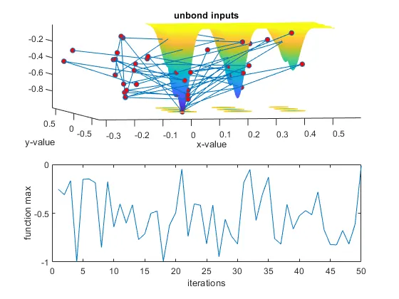
In this above graph we see that the inputs are boundless GA algorithem has mapped local maxima points out side of stalagmite functiion.

Study 2 - statistical behavior - with upper and lower bounds:-

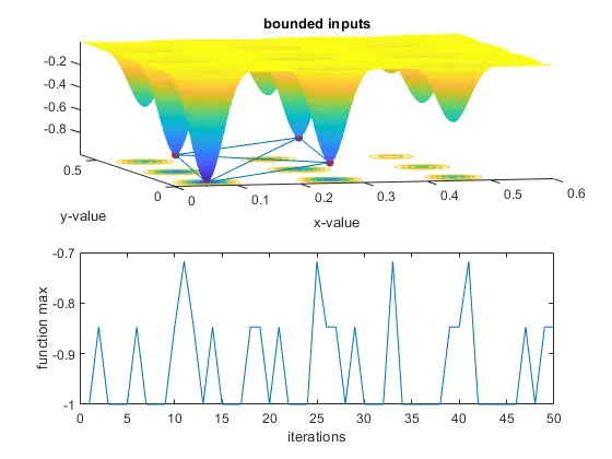
In this above graph we see that it is more clear and optimised compare to the 1st Study. The bonds are defined and we get the values in our range.

Study 3 - increasing the size of population:-

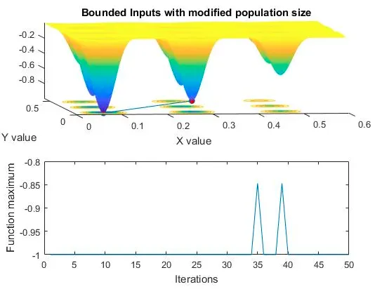
In this above graph we see that the optmise value of global maxima with accurate range.

Main Code Explanation:-

1.Program start with clear all, close all, clc.

2.Then define x and y values by using linspace command.

3.Then define the valus of num_case

4.Then 2D grid is made by using misgrid command.

5.Then the length of row and columns are used as counters.

6.Then the input vactor is declared as GA requires input vactor which is each value

7.Then output of stalagmite function is stored in matrix.

8.Then tic command is used to start a timer.

9.Then for loop bounded by the number of iterations is formed.

10.Then Study 1 - statistical behavior for 'unbond inputs' is calculated and plot the graph.

11.Then Study 2 - statistical behavior for 'bounded inputs' is calculated and plot the graph.

12.Then Study 3 - statistical behavior for 'increasing the size of population' is calculated and plot the graph.