Week 3 - Solving second order ODEs

Aim:- To solve a second order ode function for a motion of the pendulum

bjectives:-

to write a program that solves the following ODE. This ODE represents the equation of motion of a simple pendulum with damping.

Governing Equation:-

`frac{d^2 theta}{dt^2}+frac{b}{m}frac{d theta}{t theta}+frac{g}{l}sin theta=0`

where

g = gravity in m/s2,

L = length of the pendulum in m,

m = mass of the ball in kg,

b=damping coefficient.

Now we break the ode

`theta=theta1`

`frac{d theta}{dt}=frac{d theta}{dt}= theta2` (Relation - 1)

`frac{d^2 theta}{dt^2}=frac{d}{dt}(frac{d theta1}{dt})=frac{d}{dt}theta2` (Relation - 2)

Then

`frac{d^2 theta}{dt^2}+frac{b}{m}frac{d theta}{t theta}+frac{g}{l}sin theta=0`

`frac{d^2 theta1}{dt^2}+frac{b}{m}frac{d theta}{t theta}+frac{g}{l}sin theta1=0`

`frac{d theta2}{dt}+frac{b}{m} theta2+frac{g}{l}sin theta1=0`

so

`frac{d theta1}{dt}= theta2`

`frac{d theta2}{dt}=-frac{b}{m} theta2-frac{g}{l}sin theta1`

Body of Content:-

We solve the problem by using Matlab.

We write a function cod to simplify to solve the second order ode.

Then we plot the results.

After plotting we will create an animation for the pendulum.

Matlab Program:-

clear all
close all
clc

%Inputs
b = 0.05;
g = 9.81;
l = 1;
m = 1;

%initial condition
theta_0 = [0;3];

%time points
tspan = linspace(0,20,200);

%solve ode
[t,results] = ode45(@(t,theta) ode_func(t,theta,b,g,l,m),tspan,theta_0);

figure(1)
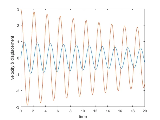
plot(t,results(:,1))
hold on
plot(t,results(:,2))
xlabel('time')
ylabel('velocity & displacement')

%Movie
ct = 1
for i = 1:length(results(:,1));
x0 = 0;
y0 = 0;
x1 = l*sin(results(i,1)+pi)
y1 = l*cos(results(i,1)+pi)

figure(2)
plot([x0 x1],[y0 y1],'-o','markersize',10,'markerfacecolor','r','markeredgecolor','r','linewidth',3)
axis([-2 2 -2 2])
hold on
plot([-1 1],[0 0],'linewidth',5,'color','[0 0.3 0]')
M(ct) = getframe(gcf)
hold off
ct = ct+1;
end

movie(M)
video_file = VideoWriter('Pendulum_motion.avi')
open(video_file)
writeVideo(video_file,M)
close(video_file)

Code explanation:-

Start the program by using clear all, close all, clc command

Then mention all the inputs.

Then solve by using ode45 matlab inbuilt command with function command.

By using plot command graph vrlocity and displacement against time.

By using for loop command create a graph for mass at various points and time.

By using movie command create an animation movie.

Function Code:-

function [dtheta_dt] = ode_func(t,theta,b,g,l,m)

theta1 = theta(1)
theta2 = theta(2)
dtheta1_dt = theta2;
dtheta2_dt = -(b/m)*theta2 - (g/l)*sin(theta1);
dtheta_dt = [dtheta1_dt; dtheta2_dt];
end

Code explanation:-

In function code the second order ode is simplified using first order ode through theta1 and 2

Then theta1 and 2 is differentiated.

Then the dtheta_dt is given in a column matrix.

Graph:-

Animation:-

https://www.youtube.com/watch?v=9y-IxHmhJUw

Conclusion:-

Hear is the simulation of the pendulum motion, by using second order ode.