Week 4.1 - Genetic Algorithm

OPTIMISATION OF STALAGMITE FUNCTION AND FIND THE GLOBAL MAXIMA OF THE FUNCTION USING GENETIC ALGORITHAM IN MATLAB

AIM:

To create code in MATLAB to optimize the stalagmite function and find global maxima of the function using genetic algorithm

GOVERNING EQUATION:

`f(x,y)=f_(1,x) f_(2,x) f_(1,y) f_(2,y)`

`f_(1,x)=[sin(5.1*π*x+0.5)]^6`

`f_(1,y)=[sin(5.1*π*y+0.5)]^6`

`f_(2,x)=exp[-4*ln(2)[(x-0.0667)^2/0.64]`

`f_(2,y)=exp[-4*ln(2)[(y-0.0667)^2/0.64]`

OBJECTIVE:

1. To define the stalagmite function
2. To find the optimum value of the stalagmite function using various method
3. To explain the concept of genetic algorithm
4. To find the global maxima value

• Statistical behavior with unbound method
• Statistical behavior with bounds method
• Statistical behavior with bounds and population size method

ABOUT GENETIC ALGORITHAM:

Nature has always been a great source of inspiration to all mankind . Genetic algorithm(GA) are search based algorithm based on the concepts of natural selection and genetics. GA are the concept of much larger branch of computation knoen.

GA are developed by John holland and his students and colleagues at the university of Michigan ,most notably David E. Goldberg and his since been tried on various optimization problems with a high degree of success

In GA, wee have a pool or a population of possible solution to the given problem. These solution then undergoes recombination and mutation ,producing new children and process is repeated various generations. Each individual is assigned a fitness value and the fitter individual are given a higher chance to mate and yield more ‘fitter’ individual .This is in line with the Darwinian theory of ‘survival of the fittest’

In this way we keep ‘evolving ‘ better individuals or solutions over generation ,ti;; we reach a stopping criterion

Genetic algorithm are sufficient randomized in natural , but they perform much better than random local search (in which we try various random solutions ,keep track of the best so far)aas they exploit historical information as well.

CONCEPT OF GENETIC ALGORITHM:

Genetic algorithm is a research based optimization technique based on the principles of ‘Genetic natural selection’. It is frequently useded to find optimal or near-optimal solution to difficult problem which otherwise would take a lifetime to solve .it is frequently used to solve optimal problems.in research , and in machine learning .we need to choose an optimal algorithm is one of the optimization processes.

The following flow chart shows how genetic algorithm work

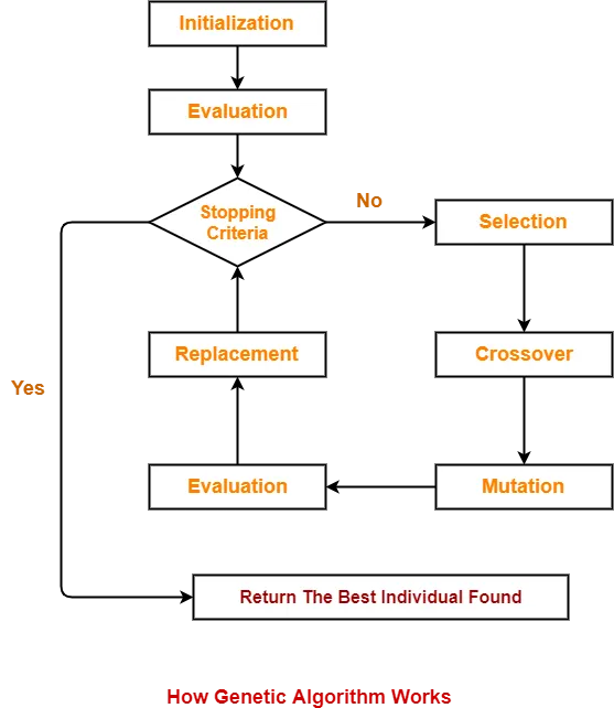
Five phase are considered in genetic algorithm

1. Initial population
2. Fitness function
3. Selection
4. Crossover
5. Mutation

INITIAL POPULATION:

The process begins with a set of individuals which is called a population .Each individual is a solution to the problem you want to solve.

FITNESS FUNCTION:

The fitness function determine how fit an individual is(the ability of an individual to compete with other individual) . is gives a fitness score to each individual . the probability that an individual will be selected for reproduction Is based on the fitness value .

SELECTION:

The idea of selection phase is to select the fittest individuals and let them pass their genes to them next generation .

CROSS OVER:

Crossover is the most significant phase in a genetic algorithm . For each pair of parent to be mated , a crossover point is chosen at random from with in the genes.

MUTATON:

In certain new offspring formed ,some of their can be subjected to mutation with a low random probability .this implies that some of the of the bit in string can be flipped.

CODE:

STALAGMITE FUNCTION:

function [f]=stalagmite(input_vector )


term1=(sin(5.1*pi*input_vector(1)+0.5))^6;
term2=(sin(5.1*pi*input_vector(2)+0.5))^6;
term3=exp(-4*log(2)*((input_vector(1)-0.0667)^2)/0.64);
term4=exp(-4*log(2)*((input_vector(2)-0.0667)^2)/0.64);
[f]=-term1*term2*term3*term4;

end

Statistical behavior with unbound method:

  clear all 
close all
clc
%define our search space 
x=linspace(0,0.6,150);
y=linspace(0,0.6,150);

%creating a two dimension array
[xx, yy]=meshgrid(x,y);
%evaluating the stalagmite function
for i=1:length(xx)
    for j=1:length(yy)
        input_vector(1)=xx(i,j);
        input_vector(2)=yy(i,j);
        f(i,j)=stalagmite(input_vector);
    end
end
num_cases=50
%study 1_satistical behavior
%iteration time
tic
for i=1:num_cases
    [inputs,fopt(i)]=ga(@stalagmite,2);
    xopt(i)=inputs(1);
    yopt(i)=inputs(2);
end

study1_time=toc
figure(1)
subplot(2,1,1)
hold on
surfc(x, y, -f)

shading interp
plot3(xopt,yopt,-fopt,'marker','o','markersize',5,'markerfacecolor','r')
title('unbounded input')
subplot(2,1,2)
plot(-fopt)
xlabel('Iteraiion')
ylabel('Function maximum')

Statistical behavior with bounds method:

clear all 
close all
clc
%define our search space 
x=linspace(0,0.6,150);
y=linspace(0,0.6,150);

%creating a two dimension array
[xx, yy]=meshgrid(x,y);
%evaluating the stalagmite function
for i=1:length(xx)
    for j=1:length(yy)
        input_vector(1)=xx(i,j);
        input_vector(2)=yy(i,j);
        f(i,j)=stalagmite(input_vector);
    end
end
num_cases=50
%study 2_satistical behavior
tic
for i=1:num_cases
    [inputs2,fopt2(i)]=ga(@stalagmite,2,[],[],[],[],[0;0],[1;1]);
    xopt2(i)=inputs2(1);
    yopt2(i)=inputs2(2);
end

study2_time=toc
figure(2)
subplot(2,1,1)
hold on
surfc(x, y, -f)

shading interp
plot3(xopt2,yopt2,-fopt2,'marker','o','markersize',5,'markerfacecolor','r')
title('bounded input')
subplot(2,1,2)
plot(-fopt2)
xlabel('Iteraiion')
ylabel('Function maximum')

Statistical behavior with bounds and population size method:

clear all 
close all
clc
%define our search space 
x=linspace(0,0.6,150);
y=linspace(0,0.6,150);

%creating a two dimension array
[xx, yy]=meshgrid(x,y);
%evaluating the stalagmite function
for i=1:length(xx)
    for j=1:length(yy)
        input_vector(1)=xx(i,j);
        input_vector(2)=yy(i,j);
        f(i,j)=stalagmite(input_vector);
    end
end
num_cases=50
%study 3_satistical behavior
options=optimoptions('ga')
options=optimoptions(options,'PopulationSize',300);
tic
for i=1:num_cases
    [inputs3,fopt3(i)]=ga(@stalagmite,2,[],[],[],[],[0;0],[0.2;0.2],[],[],options);
    xopt3(i)=inputs3(1);
    yopt3(i)=inputs3(2);
end

study3_time=toc
figure(3)
subplot(2,1,1)
hold on
surfc(x, y, -f)

shading interp
plot3(xopt3,yopt3,-fopt3,'marker','o','markersize',5,'markerfacecolor','r')
title('bounded input with polulation')
subplot(2,1,2)
plot(-fopt3)
xlabel('Iteraiion')
ylabel('Function maximum')

CODE EXPLANATION :

1. Give the range of x and y value in ‘linspace’ command to get a value in matrix
2. Use the ‘meshgrid’ command to get a matrix vaoue of xx and yy
3. Use ‘for’ loop to finding the stalagmite function value for x and y values.
4. In for loop to calling the ‘ stalagmite function program’ for finding the f values (use -ve sign to find the global maxima)
5. After finding the function value (f value) use surf to plot the values.
6. Using ‘shade interp ‘ to hide the lines in the stalagmite plot.
7. Use ‘ga ‘ to find the global maxima and minima l, local maxima and minima in the stalagmite function. In MATLAB ga will give only minima value
8. Give ‘num_cases’ value to run the number of ga iteration.
9. In study 1 – Statistical Behaviour webget ‘unbounded inputs ‘ using the ga syntax of x= ga ( fun, nvars); and finding the xopt, yopt, values using for loop
10. Use ‘subplot’ to get two plots in a single figure.
11. Use ‘plot3’ command to plot three values in a single plot.
12. Use onother ‘subplot’ to get another plot in a above figure (1) window.
13. Use plot command to plot the -fopt value in figure (1) window.
14. Use xlabel ylabel to command the name of xvalues and y values
15. Use tic and toc command to calaculate the time of getting output for study 1
16. In study 2- statistical behavior with upper and lower bounds we get the ‘bounded inputs’ and finding the xopt, yopt values using ‘for loop’.
17. Use subplot plot 3 plot xlabel ylabel tic and toc command similary to study 1.
18. In study 3 -Increasing GA iterations we get the ‘Global maxima’ using the ga syntax of x.
19. Use subplot plot 3 plot xlabel ylabel tic and toc command similary to study 1 And study 2.
20. Use fprintf command to get the function value and the function value must be in postive because we are finding the global maxima values.
21. Finally prews the run button to run the program and getting the output of global maxima.

RESULTS:

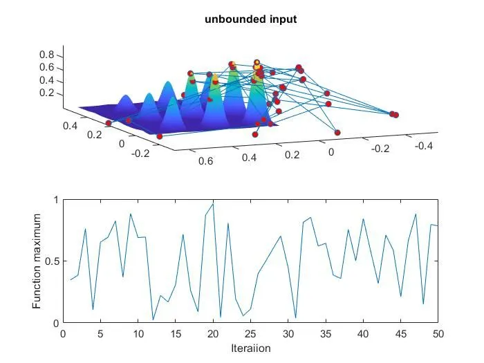
Statistical behavior with unbound method:

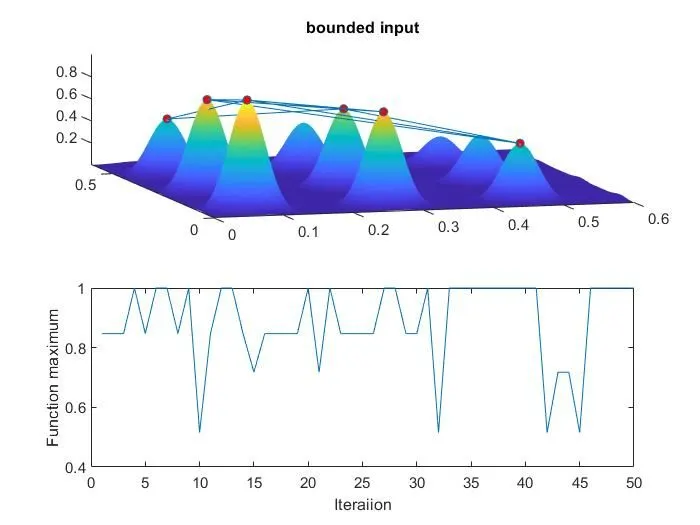
Statistical behavior with bounds method:

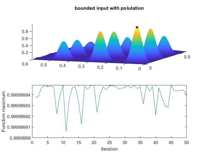
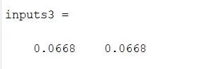
Statistical behavior with bounds and population size method:

CONCLUSIONS:

Hence we are able to optimise the stalagmite function and find the global maxima of the function

The GA is only used for the minimum function therefore to maximize the function we inversed the minimum function.