Project 2 - Rankine cycle Simulator
Rankine cycle Simulator using MATLAB
INTRODUCTION:
In many industries and research laboratories, it is often needed to exchange information between different departments. In some cases, testing may be conducted in a different location and the back end team could be asked to read and interpret the data. In such situations, parsing the data is essential to extract only relevant information, which can be used for further analysis. Therefore, file parsing is a very important procedure to learn and understand.
AIM:
The primary goal of this project is to parse one of NASA's thermodynamic data set, which contains polynomial coefficients for calculation of specific heat at constant pressure, enthalpy and entropy. In addition, the molecular weight of all the species is calculated.
OBJECTIVE:
The main objectives of this project are to.
(1) learn the underlying procedure of the file parsing.
(2) write a MATLAB code to parse a Thermodynamic data file from NASA .
(3) Run the file parsing code for multiple species (i.e. chemical compounds) provided in the Thermodynamic data file .
(4) Calculate the Cp, enthalpy and entropy for the different temperature ranges.
(5) Interpret the results for O2, N2 and CO2 species (vi) Automatically save the plots in appropriate species folders.
THEORY:
RANKINE CYCLE:
The Rankine cycle or Rankine Vapor Cycle is the process widely used by power plants such as coal fired power plants or nuclear reactors. In this mechanism, a fuel is used to produce heat within a boiler, converting water into steam which then expands through a turbine producing useful work.
components used:
1) Turbine 2) Condenser 3) Pump 4) Boiler
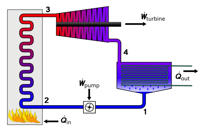
The efficiency of the Rankine cycle is limited by the high heat of vaporization by the fluid. The fluid must be cycled through and reused constantly, there for, water is the most practical fluid for this cycle. This is not why many power plants are located near a body of water-that's for the waste heat. As the water condenses in the condenser, waste heat is given off in the form of water vapour-which can be seen billowing from a plant's cooling towers. This waste heat is necessary in any thermodynamic cycle. Due to this condensation step, the pressure at the turbine outlet is lowered. This means the pump requires less work to compress the water-resulting in higher overall efficiencies.
process include in rankine cycle:
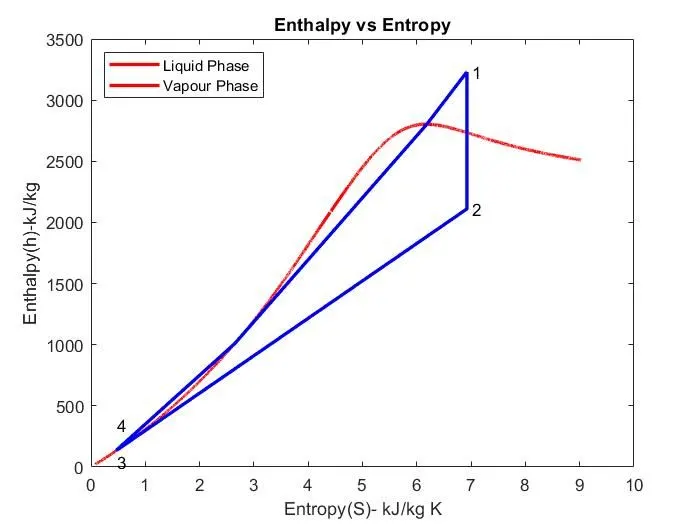
1-2 process: isentropic expansion in turbine.
2-3 process: constant pressure heat rejection in condenser.
3-4 process: isentropic compression using pump.
4-1 process: constant pressure heat addition in boiler.
FORMULA USED:
T4 = T1s/exp((s1f-s4)/high_cpl);
Wnet = Wt - Wp
B.W.R = -Wp/Wt
Efficiency =Wnet*100/Qin
high_cpl = specific heat constant of fluid at p1
where,
T4 = temperature at the inlet of the boiler.
T1s = temperature at the saturation line of state1
s1f = fluid entropy at the inlet of turbine
s4 = entropy of fluid at the inlet of boiler
high_cpl = specific heat constant of fluid at p1
Wnet -net work done
B.W.R = back work ratio
Wp = work done by pump
Wt = work done by turbine
Qin =heat addition to the fluid in boiler
CODE:
clear all
close all
clc

disp('Rankine Cycle Simulator')
disp('process 1-2: Isentropic expansion in turbine ')
disp('process 2-3: constant pressure heat rejection in condenser')
disp('process 3-4: Isentropic Compression in pump')
disp('process 4-1: constant pressure heat addition in boiler')

% Intial data inputs
T1 = input('Enter the turbine inlet temp: ');
p1 = input('Enter the turbine inlet press: ');
p2 = input('Enter the turbine outlet press: ');


% State Point 1 parameters i.e Turbine Inlet
Tsat = XSteam('Tsat_p',p1);
h1 = XSteam('h_pt',p1,T1);
s1 = XSteam('s_pt',p1,T1);

%State Point 2 parameters i.e Condenser Inlet
s2 = s1;
sf2 = XSteam('sL_p',p2);
sg2 = XSteam('sv_p',p2);

% s2=sf2+(x2*sfg2)
% Dryness fraction
x2 =(s2-sf2)/(sg2-sf2);

T2 = XSteam('T_ps',p2,s2);
h2 = XSteam('h_px',p2,x2);
hf2 = XSteam('hL_p',p2);

% State Point 3 Parameters i.e Pump Inlet
p3 = p2;
T3 = T2;
s3 = sf2;
h3 = hf2;
T5 = Tsat;

% State Point 4 Parameters i.e Boiler Inlet
s4 = s3;
p4 = p1;
h4=XSteam('h_ps',p4,s4);
cp=XSteam('cp_ps',p4,s4);
cv=XSteam('cv_ps',p4,s4);
c=cp/cv;
T4=T3*((p4/p3)^(c-1)/c)

% State Point 5,6 Parameters
T5=Tsat;
h5=XSteam('hL_p',p1);
s5=XSteam('sL_p',p1);
T6=T1;
h6=XSteam('hV_p',p1);
s6=XSteam('sV_p',p1);

% Plotting T-S Diagram
t=linspace(5,400,25000);
for i=1:length(t)
s(i)=XSteam('sL_t',t(i));
S(i)=XSteam('SV_t',t(i));
h(i)=XSteam('hL_t',t(i));
H(i)=XSteam('hV_t',t(i));
end
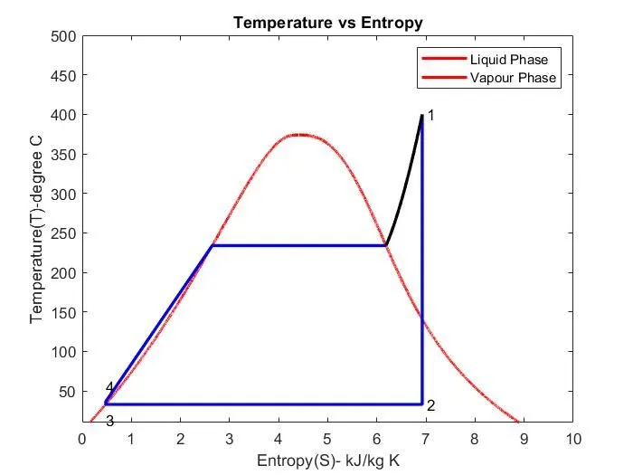
figure(1)
plot(s,t,'color','r','linewidth',2);
hold on
plot(S,t,'color','r','linewidth',2);

%ploting T vs s
plot([s1,s2,s3,s4,s5,s6],[T1,T2,T3,T4,T5,Tsat],'linewidth',2,'color','b');
text(s1+0.1, T1, '1')
text(s2+0.1, T2, '2')
text(s3, T3-20, '3')
text(s4, T4+20, '4')
axis([0,10,10,500]);


% Plotting Saturated Temperature
a=linspace(Tsat,T1,500);
for i=1:length(a)
    d(i)=XSteam('s_pt',p1,a(i));
end
plot(d,a,'linewidth',2,'color','k')
title('Temperature vs Entropy')
xlabel('Entropy(S)- kJ/kg K')
ylabel('Temperature(T)-degree C')
legend('Liquid Phase','Vapour Phase')


figure(2)
plot(s,h,'color','r','linewidth',2);
hold on
plot(S,H,'color','r','linewidth',2);
%PLOTING h VS S
plot([s1,s2,s3,s4,s5,s6,s1],[h1,h2,h3,h4,h5,h6,h1],'linewidth',2,'color','b');
text(s1+0.1, h1, '1')
text(s2+0.1, h2, '2')
text(s3, h3-100, '3')
text(s4, h4 +200, '4')
title('Enthalpy vs Entropy')
xlabel('Entropy(S)- kJ/kg K')
ylabel('Enthalpy(h)-kJ/kg')
legend('Liquid Phase','Vapour Phase','location','northwest')

% Result to be displayed in the command window
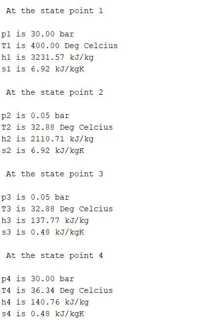
disp(' The following are the results of rankine cycle operation ')
disp(' ')
disp(' At the state point 1')
disp(' ')
n1=sprintf('p1 is %.2f bar',p1);
disp(n1)
n2=sprintf('T1 is %.2f Deg Celcius',T1);
disp(n2)
n3=sprintf('h1 is %.2f kJ/kg',h1);
disp(n3)
n4=sprintf('s1 is %.2f kJ/kgK',s1);
disp(n4)

disp(' ')
disp(' At the state point 2')
disp(' ')
n5=sprintf('p2 is %.2f bar',p2);
disp(n5)
n6=sprintf('T2 is %.2f Deg Celcius',T2);
disp(n6)
n7=sprintf('h2 is %.2f kJ/kg',h2);
disp(n7)
n8=sprintf('s2 is %.2f kJ/kgK',s2);
disp(n8)

disp(' ')
disp(' At the state point 3')
disp(' ')
n9=sprintf('p3 is %.2f bar',p3);
disp(n9)
n10=sprintf('T3 is %.2f Deg Celcius',T3);
disp(n10)
n11=sprintf('h3 is %.2f kJ/kg',h3);
disp(n11)
n12=sprintf('s3 is %.2f kJ/kgK',s3);
disp(n12)

disp(' ')
disp(' At the state point 4')
disp(' ')
n13=sprintf('p4 is %.2f bar',p4);
disp(n13)
n14=sprintf('T4 is %.2f Deg Celcius',T4);
disp(n14)
n15=sprintf('h4 is %.2f kJ/kg',h4);
disp(n15)
n16=sprintf('s4 is %.2f kJ/kgK',s4);
disp(n16)

% Workdone by turbine

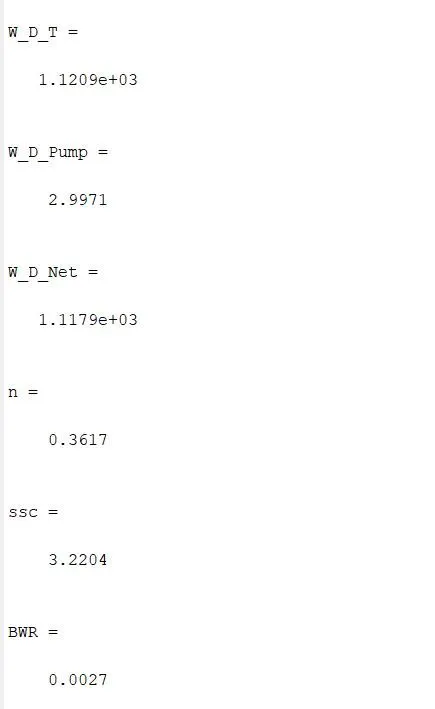
W_D_T = h1-h2

% Workdone by the pump

W_D_Pump = h4-h3

%net workdone

W_D_Net = W_D_T-W_D_Pump

% Heat Supplied
q = h1-h4;

% Effeciency
n = W_D_Net/q

% Specific steam consumption
ssc = 3600/W_D_Net

% Back Work Ratio
BWR = W_D_Pump/W_D_T
CODE EXPLANATION:
- First of all, set the input variables p1, T1, and p2 using input command.
- Calculating the variables at state 1,2, 3 and 4 state using the XSteam which is having all values of steam table file.
- Plot the H-S curve using plot command.
- The saturation curve can be plotted by dividing the temperature into parts up to 373K(which is critical temperature of water) and finding the value of enthalpy and Entropy for liquid and vapour for the above defined range of temperature.
- Plot the saturation line using plot command.
- Plotting T-S curve and saturation curve in figure 2
- Calculating network, back work ratio an efficiency using the above formulas.
RESULTS:
PLOT:
TEMPERATURE VS ENTROPY:
ENTHALPY VS ENTROPY :
CONCLUSION:
In this project, the procedure of file parsing was well understood. In addition, using if statements and for loops as needed to optimize the code was a good learning experience. This knowledge can be used to parse any data file and extract relevant information as needed. As a future work, the calculated molecular weights can be written out to a text file for reference and comparison. Any chemical compound can be tracked and studied. The file parsing code has to be tailored to suit the input data file.