Project 1 - Parsing NASA thermodynamic data

PARSING NASATHERMODYNAMIC DATA USING MATLAB

AIM :

To write a MATLAB program to extract 14 coefficients from the MATLAB extract THERMO.dat.txt file to calculate enthalpy, entropy, specific heat, for all the species in the data file. Also by plotting graphs of every species and find the molecular mass of the species.

OBJECTIVE :

1. To write a function that extracts 14 co-efficient for a given species from the given information.
2. To write functions that calculate the enthalpy, entropy, and specific heat using NASA polynomials for the given species.
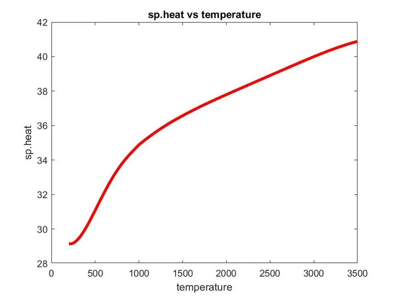
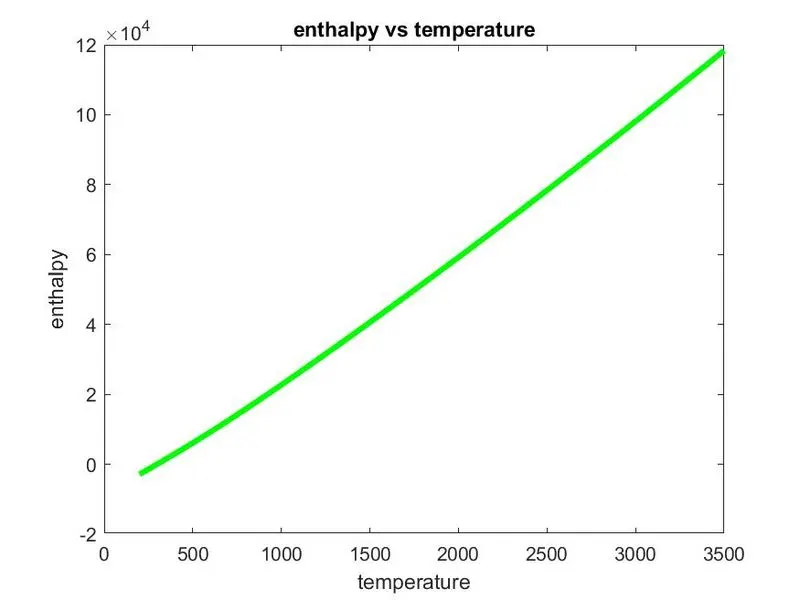
3. To write a function that plots the Cp, Enthalpy, and Entropy of input species.
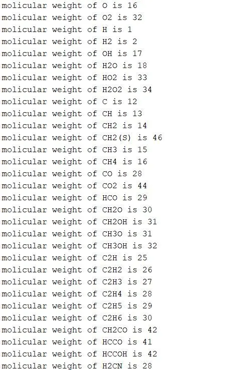
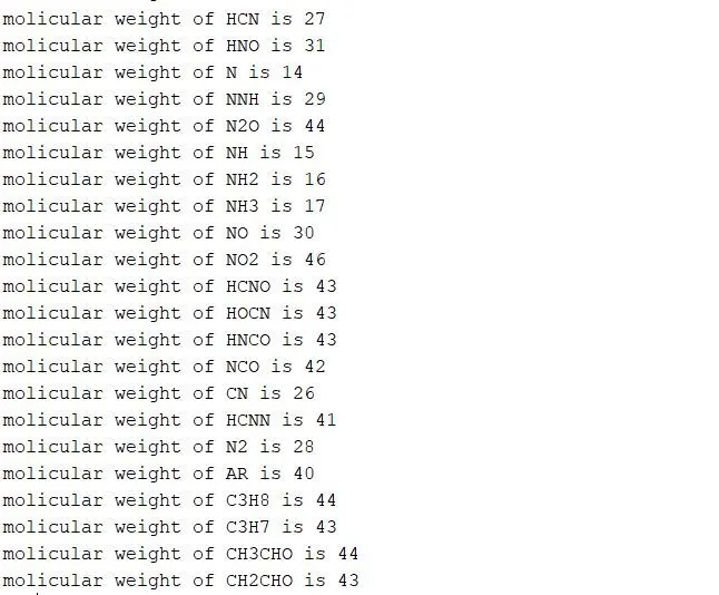
4. To write a function that calculates the molecular weight of each species.

INTRODUCTION :

File parsing is done to extract data from the file, it should be generic as possible to fetch the data and by using this we calculate enthalpy, entropy & specific heat for different species and condition is that the first 7 coefficients are high temperature coefficient & second 7 coefficient are low temperature coefficient.

Parsing can be defined as of breaking the data block into smaller blocks by following set of orders. So that it can be more easily interpreted, managed and sent to a computer NASA came up with the polynomials that can be used to evaluate thermodynamic properties such as Cp, Enthalpy, and Entropy using polynomials. They have also documented the co-efficient that are required to evaluate these polynomials for 1000+ species. The formulas to calculate Cp, Enthalpy, and Entropy are given below,

(Cp)/R = a1 + a2*T + a3*T^2 + a4*T^3 + a5*T^4

(H)/RT = a1 + a2*T/2 + a3*T^2/3 + a4*T^3/4 + a5*T^4/5 + a5*T

(S)/R =a1*1n(T) + a2*T + a3*T^2 /2+ a4*T^3/3 + a5*T^4/4 + a7

THEORY :

File parsing refers to how information can be read or extracted form a particular file and how the information can be used in a computer program. With the help of file parsing we can read data from external files and data bases and we use that information or data in our calculations.

SPECIFIC HEAT CAPACITY :

The specific heat of a substance is defined as the amount of heat required to raise a unit mass of a substance through a unit rise in temperature. however it would be pretty in convenient to measure the heat capacity of every unit of matter. What we want is an intensive property that depends only on the type and phase of a substance and can be applied of systems of arbitrary size. This quantity is known specific heat capacity. Experiments show that the transferred heat depends on three factors.

1. The change in temperature.
2. The mass of the system
3. Substance and phase of the system.

Q = mcT

Where Q is heat transfer, m Is the mass of the substance, T is the temperature change, c stands for specific heat capacity.

ENTHALPY :

The enthalpy of a substance, h is defined as h = u + pv

U is the internal energy, p and v are the pressure and volume of the system. The state off the gas is defined by several properties including the temperature l, pressure, and volume which gas occupies.

From the study of the first law of thermodynamics we find the internal energy of a gas is also a state variable that is a variable depends only on the state of a gas and not on any process that produced that state.

ENTROPY :

Generally entropy is defined as a measure of randomness or disorder of a system. This concept was introduced by a German physicist named rudolf clausius in 1850. From the thermodynamic view point entropy is used to describe the behaviour of a system in terms of thermodynamic property such as temperature, pressure, and heat capacity. This thermodynamic description take in to consideration the state of equilibrium of the system .Entropy is an extensive property increases with decreases with regularity.

The change in entropy,

S = (Q/T)

Where Q is heat transfer, T is the absolute temperature

PROCEDURE:

1. All the extra windows and old data is cleared with the help of clear all, close all, clc
2. Then we read THERMO.DAT.txt file to calculate Enthalpy, Entropy & Specific heat.
3. To read the file we assigned to a variable called fin order to get data with respect to global temperature, local temperature & calculation of coefficients thermodynamic properties.
4. To access the next line we have used the command fgetL
5. First value of temperature is converted with the help of string 2 number(str2num) command so that the no in " can be converted into plain number.

6. Now we have assigned temperatures to the global low temperature, global high temperature & global medium temperature
7. Now as shown in the figure the lines are not useful so to neglect these lines we have used for loop 1:3 to skip these 3 lines
8. To split the given value in line we have used strsplit.
9. Then we have calculated value for species
10. Now to convert local temperatures into double precision values and to convert the complex number into cell array/string array we will use str2double command.
11. Now to Store the values of the second line of variables we will use fgetl command here also but assign it to the line
12. And to find the value (string) of that particular line now we will use strfind command.
13. Now again by using str2double command we will find 14 coefficients for all the species.
14. First 7 species are of high temperature coefficients & next 7 are of lower temperatures.
15. Now we will define higher and lower temperatures with the help of linspace Command.
16. Now we will calculate Cp, h, & S for lower and higher temperature limits.
17. We assumed universal gas constant R as 8.134 & also in the above linspace commands we have defined our temperature ranges

18. After putting all the values of a in respective commands of enthalpy. entropy and specific heat wwe have to plot the graphs to see the nature of the graphs and their values.
19. To do this in this project we have to Make Folders for saving the plots so the current_dir opens present working directory and the mkdir command makes the new folder with the name specified inside brackets.
20. A folder named NASA F1 graphs created in the working directory which is used to store all the related data of output files of the program.
21. Command cd makes new folder as the directory which is used for storing all related output files of the program.
22. After program get executed the cd(current_dir) command helps to return to the original directory

CODE :

clear all
close all
clc
%file reading
f1=fopen('THERMO.dat','r');
fgetl(f1);
%get first line
tline1=fgetl(f1);
b=strsplit(tline1,' ');
%store global temperature
global_low_temp=str2num(b{1})
global_mid_temp=str2num(b{2})
global_high_temp=str2num(b{3})
R=8.314
for i=1:3
    fgetl(f1);
end
for i=1:53
tline2=fgetl(f1);

%split srring at space
b1=strsplit(tline2,' ');
species_name=b1{1};
m=length(b1);
local_low_temp=str2num(b1{m-3});
local_mid_temp=str2num(b1{m-1});
local_high_temp=str2num(b1{m-2});
%local temperature of individual species
T=linspace(local_low_temp,local_high_temp,100);
%1st line
tline3=fgetl(f1);
c=findstr(tline3,'E');
a1=tline3(1:c(1)+3);
a1=str2num(a1);
a2=tline3(c(1)+4:c(2)+3);
a2=str2num(a2);
a3=tline3(c(2)+4:c(3)+3);
a3=str2num(a3);
a4=tline3(c(3)+4:c(4)+3);
a4=str2num(a4);
a5=tline3(c(4)+4:c(5)+3);
a5=str2num(a5);
%2nd line
tline4=fgetl(f1);
c=findstr(tline3,'E');
a6=tline4(1:c(1)+3);
a6=str2num(a6);
a7=tline4(c(1)+4:c(2)+3);
a7=str2num(a7);
a8=tline4(c(2)+4:c(3)+3);
a8=str2num(a8);
a9=tline4(c(3)+4:c(4)+3);
a9=str2num(a9);
a10=tline4(c(4)+4:c(5)+3);
a10=str2num(a10);
%3rd line
tline5=fgetl(f1);
c=findstr(tline3,'E');
a11=tline5(1:c(1)+3);
a11=str2num(a11);
a12=tline5(c(1)+4:c(2)+3);
a12=str2num(a12);
a13=tline5(c(2)+4:c(3)+3);
a13=str2num(a13);
a14=tline5(c(3)+4:c(4)+3);
a14=str2num(a14);

%find the enthalpy,entropy and specific heat
for i=1:100
if T(i)>=local_mid_temp;
cp(i)=R*(a1+a2*T(i)+a3*T(i)^2+a4*T(i)^3+a5*T(i)^4);
h(i)=R*T(i)*(a1+a2*T(i)/2+a3*(T(i)^2)/3+a4*(T(i)^3)/4+a5*(T(i)^4)/5+a6/T(i));
s(i)=R*(a1*log(T(i))+a2*T(i)+a3*(T(i)^2)/2+a4*(T(i)^3)/3+a5*(T(i)^4)/4+a7);

else T(i)<local_mid_temp;
cp(i)=R*(a8+a9*T(i)+a10*T(i)^2+a11*T(i)^3+a12*T(i)^4);
h(i)=R*T(i)*(a8+a9*T(i)/2+a10*(T(i)^2)/3+a11*(T(i)^3)/4+a12*(T(i)^4)/5+a13/T(i));
s(i)=R*(a8*log(T(i))+a9*T(i)+a10*(T(i)^2)/2+a11*(T(i)^3)/3+a12*(T(i)^4)/4+a14);
end
end
%for store the plots in NASA F1 folder
mkdir(['C:\Users\USER\Desktop\matlab trial\NASA F1'],species_name);
cd(species_name);

%plot sp.heat vs temperature
figure(1)
plot(T,cp,'linewidth',3,'color','r')
xlabel('temperature')
ylabel('sp.heat')
title('sp.heat vs temperature')
saveas(figure(1),'cp.jpg')

%plot enthalpy vs temperature
figure(2)
plot(T,h,'linewidth',3,'color','g')
xlabel('temperature')
ylabel('enthalpy')
title('enthalpy vs temperature')
saveas(figure(2),'h.jpg')

%plot entropy vs temperature
figure(3)
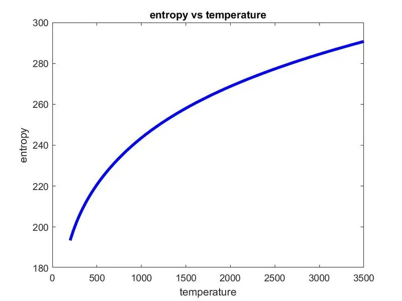
plot(T,s,'linewidth',3,'color','b')
xlabel('temperature')
ylabel('entropy')
title('entropy vs temperature')
saveas(figure(3),'s.jpg')

%for finding molicular mass
element=['H','O','C','N','S','A'];
atomic_wt=[1 16 12 14 32 40];
mw=0;
for i=1:length(species_name)
    for j=1:length(atomic_wt)
        if strcmp(species_name(i),element(j))==1;
            mw=atomic_wt(j)+mw;
            v=j;
        end
    end
    n=str2num(species_name(i));
    if n>1
        mw=atomic_wt(v)*(n-1)+mw;
    end
end
fprintf('molicular weight of %s is %d\n',species_name,mw)


cd ..


end
fclose(f1);

CODE EXPLANATION :

• To start with we open the thermodynamic file THERMO. Dat and the data in the file is bieng read with the help of fopen command
• Following this we read the Heading of the file with help of fgetl command reading the first line.
• Whenever we use fgetl command after this point, the command will read the next line. So using fgetl again we read the Global temperature and they are converted to number from string with the help of str2num command.
• Using strsplit command we extract the read global low, mid and high temperature given in the file.
• At this point we need to skip next 3 lines and this is done by using fgetl command again for 3 times.
• Following this next we have to extract the coefficients which are specific for each species. This is done by using for loop. We run the loop 53 times as we have 53 different species in the file.
• Within the loop we read and exctracted the local temperature for each species. This is important as new can to calculate the thermodynamic properties. Using the local low, mid and high temperature.
• Using findstr command we specifically found out the number of exponiential in the first line of coefficients and accordingly extracted the number of coefficients.
• This is done of the all the coefficients carrying line separately.
• The coefficients which are bieng extracted are in string form and are converted to number with str2num command
• Once we extracted all rhe coefficients next we have to calculate the thermodynamic properties ie specific heat(Cp), Enthalpy (H), Entropy(S). We calculated these properties with the formula given above and substitute d the extracted coefficients im the formula.
• The first 7 coefficients are high temp.Coefficients amd the next 7 are low temp. Coefficients. So to calculate the properties specifically for high temperature and loe temperature again for loop is used and distinguished using if condition statement.
• The value of gas constant is taken as 8.322 and temperature range is taken from low temperature to high temperature with 100 valued between them.
• Following the calculation of the thermodynamic properties, the current directory is changed to the new directory which will be made for each species with that specific name.
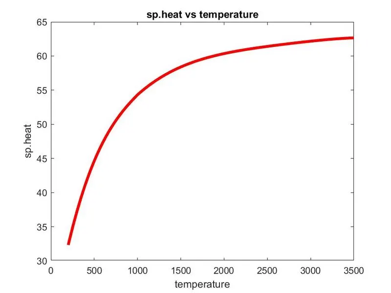
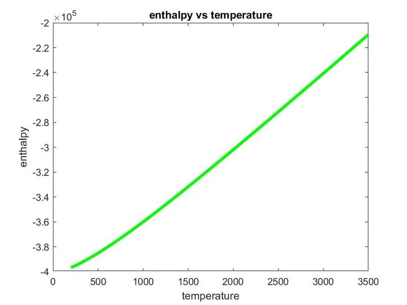
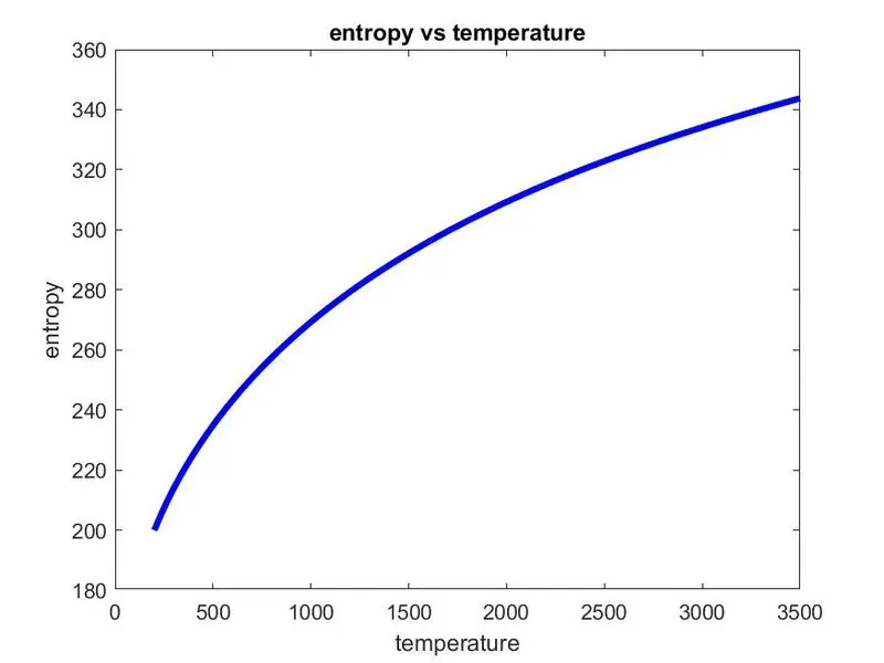
• Now we will plot the graphs specific heat vs Temperature Enthalpy vs Temperature and Entropy vs Temperature for each species using plot command. These plots are saved and dumped in the separate directory folder with their name as mentioned in the last step.
• Cd command is used to get back in the orginal directory
• Following the calculation of the thermodynamic properties, Molecular wieght of each species is calculated
• And finally we close the THERMO.dat file using fclose command.

RESULT AND PLOT :

Molicular weight of species:

PLOT OF O2:

PLOT OF N2:

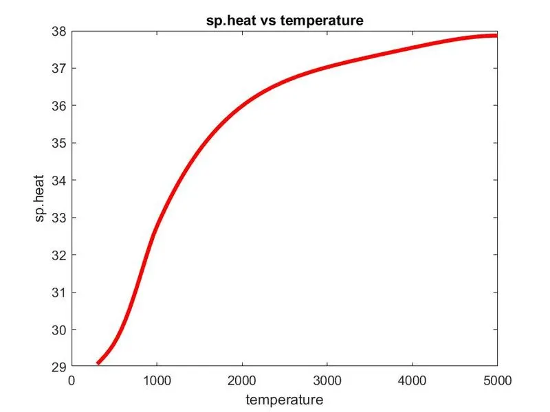
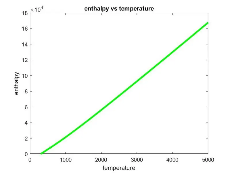
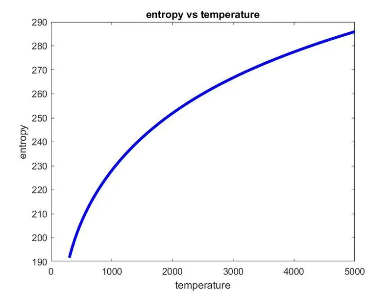
PLOT OF CO2 :

FOLDER:

CONCLUSION :

The file parsing of NASA thermodynamic data includes several modules & we converted them all into useful form, plotting the relations & saving them automatically into required current location. The different plot for each element shows the relation& trend between thermodynamic properties like Enthalpy, Entropy, Specific heat with respect to temperature.

REFERANCE:

• https://in.mathworks.com/help/matlab/ref/mkdir.html?searchHighlight=mkdir&s_tid=doc_srchtitle
• https://in.mathworks.com/matlabcentral/answers/472084-how-to-parse-text-data
• https://in.mathworks.com/help/matlab/ref/fgetl.html