Week 3 - Solving second order ODEs

SOLVING SECOND ORDER ODE : SIMPLE PENDULUM

AIM:

To solve a second order ordinary differential equation in MATLAB

OBJECTIVE:

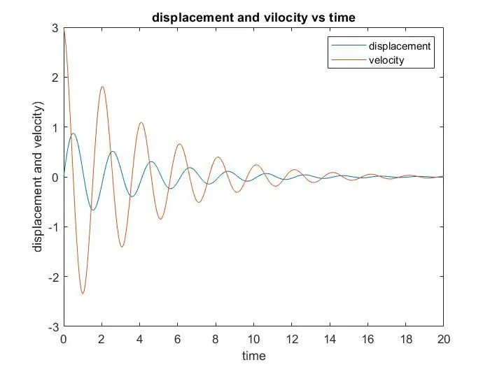
1. To solve the second order ODE in MATLAB with graph for velocity and displacement.
2. To animate the motion of simple pendulam.

GOVERNING EQUATION:

`d^2 θ/(dt)^2+(b/m)*dθ/dt+g/L*(sinθ)=0`

Where,

`θ`-angular displacement of pendulum

t- time

b-damping co_efficient

m-mass of bob

g-acceleration due to gravity

L-length of pendulum

In MATLAB, second order differential equation cannot be solved. But they can be solved by converting two first order ODE, then by using ode45 we can solve the problem.

PROCEDURE:

1. Convert the second order differential equation to first order differential equation.
2. Input the initial parameter such as length, mass ,damping co_efficient of pendulum.
3. Set the initial condition and time span for simulation.
4. Use ode45 for solving differential equation.
5. Plot the graph of displacement vs time and velocity vs time.
6. Create simulation of the position of the pendulum bob and arm using movie function.

FUNCTION CODE:

function [dtheta_dt]=ode_func(t,theta,b,g,l,m)

theta1=theta(1)
theta2=theta(2)
dtheta1_dt=theta2;
dtheta2_dt=-(b/m)*theta2-(g/l)*sin(theta1);
dtheta_dt=[dtheta1_dt; dtheta2_dt];
end

CODE EXPLANATION:

Used to convert the second order function in to two first order function.

MAIN CODE:

%simple pendulum simulation 
clear all
close all
clc

b=0.05;
g=9.81;
m=0.1;
l=1;
%initial condition
theta_t=[0;3];
%time points
t_span=linspace(0,20,300);
%solving ode
[t,results] = ode45(@(t,theta) ode_func(t,theta,b,g,l,m),t_span,theta_t);
%plot graph
figure(1)
plot(t,results(:,1));
hold on
plot(t,results(:,2));
ylabel('plot');
xlabel('time');
legend('displacement','velocity');
xlabel('time');
ylabel('displacement and velocity)');
title('displacement and vilocity vs time');

ct=1
for i=1:length(t)
    x0=0;
    y0=0;
    x1=l*sin(results(i,1));
    y1=-l*cos(results(i,1));
    %ploting line  
    figure(2)
    plot([x0 x1],[y0 y1],'linewidth',3);
    hold on
    %plote bob
    plot(x1,y1,'marker','o','markerfacecolor','r','markersize',20);
    hold off
    axis([-1 1 -1.5 0])
    pause(0.1)
     M(ct)=getframe(gcf);
    ct=ct+1;
end
%movie making and store as avi format
movie(M)
videofile = VideoWriter('project.avi','Uncompressed AVI');
open(videofile)
writeVideo(videofile,M)
close(videofile)

CODE EXPLANATION:

1. Set physical parameter of the pendulum, mass ,damping co_efficient and length.
2. Set initial condition and time span for which the ode45 have to work.
3. To solve ode, use ode45 function with main inputs as (t and theta)while you use ode_func with in put as (t,theta,l,b,m) and theta_t as initial condition.
4. These results are stored in an array of [t,results]
5. Since results contain 2 components, angular displacemet and velocity ,to plot both the graphs ,use the (:,1) and (:,2) and plot the graph.
6. To create animation use ‘for’ loop so that we can get the x and y coordinates
7. Use the pause() function to give a pause for evey looping of values.
8. Use movie making command as per code to create an animation.

PLOTE:

ANIMATION:

https://drive.google.com/file/d/1LIyfZQvtjjG53SXre9K-ULhrClFGs6Ns/view?usp=sharing

CONCLUSION:

The reduction in angle displacement and velocity is due to damping is due to the damping coefficient indroduced in the second order ODE of a simple pendulum.

We have successfully solved the second order ODE.