Week 4.1 - Genetic Algorithm

OBJECTIVE:

To write a code in MATLAB to optimize the stalagmite function and find the Global Maxima of the function using Genetic Algorithm.

THEORY:

• OPTIMIZATION:

Optimization is the selection of the best solution, with regard to some criterion, from some set of available alternatives. An optimization problem consists of maximizing or minimizing a real function by systematically choosing input values from within an allowed set and computing the value of the function.

Optimization includes finding "the best" from available values of some objective function given a defined domain(or input), including a variety of different types of objective functions and different types of domains.

An optimization algorithm is required for performing the optimization process. One such algorithm is Genetic Algorithm.

• GENETIC ALGORITHM:

Genetic Algorithm is an optimization technique inspired by the process of natural selection that belongs to the larger class of evolutionary algorithms (EA). Genetic algorithms are commonly used to generate high-quality solutions to optimization and search problems by relying on biologically inspired operators such as mutation,crossover and selection.

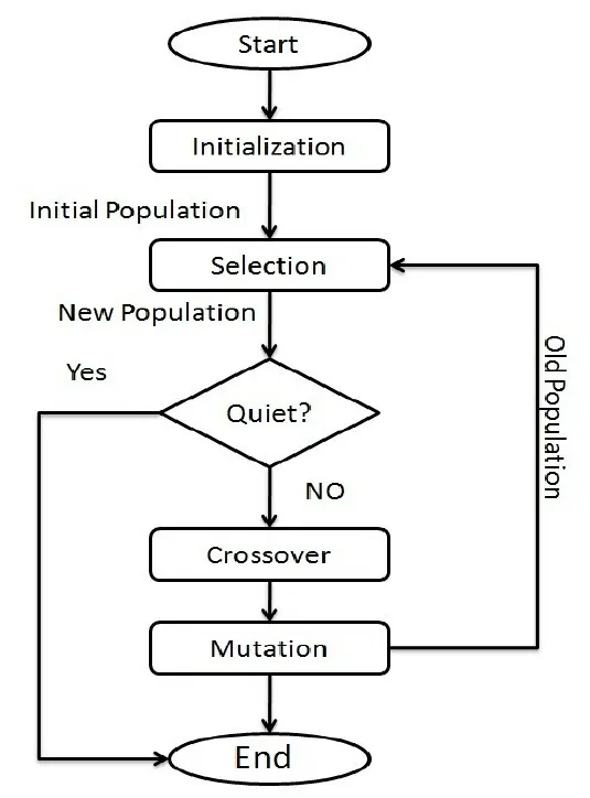
The evolution usually starts from a population of randomly generated individuals, and is an iterative process, with the population in each iteration called a generation.

• Initializaion:

In the initialization process, the population size is generated depending on the nature of problem. Higher the population size, better the results. Often, the initial population is generated randomly, allowing the entire range of possible solutions (the search space). Occasionally, the solutions may be "seeded" in areas where optimal solutions are likely to be found.

• Selection:

In this step, the "parents" are selected from the sample data points, the main objective of the selection process is to select the highly fit individual to propagate their features to the next generation. The fitness value of the given function will be computed.

• Crossover:

Crossover is a genetic operator used to combine the genetic information(chromosome) of two parents to generate new offspring. It is one way to stochastically generate new solutions from an existing population.

• Mutation:

Mutation is a genetic operator used to maintain genetic diversity from one generation of a population of genetic algorithm chromosomes to the next. Mutation alters one or more gene values in a chromosome from its initial state. In mutation, the solution may change entirely from the previous solution. Hence GA can come to a better solution by using mutation.

*These three processes (SELECTION →CROSSOVER →MUTATION) are repeated to breed new generations until an optimized solution is found.

• Termination:

This generational process is repeated until a termination condition has been reached. Common terminating conditions are:

• A solution is found that satisfies minimum criteria
• Fixed number of generations reached
• Allocated budget (computation time/money) reached
• The highest ranking solution's fitness is reaching or has reached a plateau such that successive iterations no longer produce better results
• Manual inspection
• Combinations of the above

*FITNESS FUNCTION:

Fitness Function evaluates how close a given solution is to the optimum solution of the desired problem.The fitness function should quantitatively measure how fit a given solution is in solving the problem.

SYNTAX FOR GA IN MATLAB:

(1) x = ga(fun,nvars)
(2) x = ga(fun,nvars,A,b)
(3) x = ga(fun,nvars,A,b,Aeq,beq)
(4) x = ga(fun,nvars,A,b,Aeq,beq,lb,ub)
(5) x = ga(fun,nvars,A,b,Aeq,beq,lb,ub,nonlcon)
(6) x = ga(fun,nvars,A,b,Aeq,beq,lb,ub,nonlcon,options)
(7) x = ga(fun,nvars,A,b,[],[],lb,ub,nonlcon,IntCon) or x = ga(fun,nvars,A,b,[],[],lb,ub,nonlcon,IntCon,options)
(8) x = ga(problem)
(9) [x,fval] = ga(___)
(10) [x,fval,exitflag,output] = ga(___)
(11) [x,fval,exitflag,output,population,scores] = ga(___)

DESCRIPTION:

(1) x = ga(fun,nvars) finds a local unconstrained minimum, x, to the objective function, fun. nvars is the dimension (number of design variables) of fun.

(2) x = ga(fun,nvars,A,b) finds a local minimum x to fun, subject to the linear inequalities A*x ≤ b. ga evaluates the matrix product A*x as if x is transposed (A*x').

(3) x = ga(fun,nvars,A,b,Aeq,beq) finds a local minimum x to fun, subject to the linear equalities Aeq*x = beq and A*x ≤ b. (Set A=[] and b=[] if no linear inequalities exist.) ga evaluates the matrix product Aeq*x as if x is transposed (Aeq*x').

(4) x = ga(fun,nvars,A,b,Aeq,beq,lb,ub) defines a set of lower and upper bounds on the design variables, x, so that a solution is found in the range lb ≤ x ≤ ub. (Set Aeq=[] and beq=[] if no linear equalities exist.)

(5) x = ga(fun,nvars,A,b,Aeq,beq,lb,ub,nonlcon) subjects the minimization to the constraints defined in nonlcon. The function nonlcon accepts x and returns vectors C and Ceq, representing the nonlinear inequalities and equalities respectively. ga minimizes the fun such that C(x) ≤ 0 and Ceq(x) = 0. (Set lb=[] and ub=[] if no bounds exist.)

(6) x = ga(fun,nvars,A,b,Aeq,beq,lb,ub,nonlcon,options) minimizes with the default optimization parameters replaced by values in options. (Set nonlcon=[] if no nonlinear constraints exist.) Create options using optimoptions.

(7) x = ga(fun,nvars,A,b,[],[],lb,ub,nonlcon,IntCon) or x = ga(fun,nvars,A,b,[],[],lb,ub,nonlcon,IntCon,options) requires that the variables listed in IntCon take integer values.

(8) x = ga(problem) finds the minimum for problem, a structure described in problem.

(9) [x,fval] = ga(___), for any previous input arguments, also returns fval, the value of the fitness function at x.

(10) [x,fval,exitflag,output] = ga(___) also returns exitflag, an integer identifying the reason the algorithm terminated, and output, a structure that contains output from each generation and other information about the performance of the algorithm.

(11) [x,fval,exitflag,output,population,scores] = ga(___) also returns a matrix population, whose rows are the final population, and a vector scores, the scores of the final population.

CODE:

clear all 
close all
clc

x = linspace(0,0.6,150);
y = linspace(0,0.6,150);
cases_num = 50
 
%2d Array of x and y
[xx yy] = meshgrid(x ,y);
for i = 1:length(xx)
    for j = 1:length(yy)
        input_vector(1) = xx(i,j);
        input_vector(2) = yy(i,j);
        f(i,j) = stalagmite(input_vector);
    end    
end

tic
%Study -1 Statistical Behaviour - unbounded
for i = 1:cases_num
    [inputs, fopt(i)] = ga(@stalagmite, 2);
    xopt(i) = inputs(1);
    yopt(i) = inputs(2);
end
study1_time = toc

figure(1)
subplot(2,1,1)

surfc(xx,yy,-f)
shading interp
hold on
plot3(xopt,yopt,-fopt,'marker','o','markersize',5,'markerfacecolor','r')
title('Unbounded inputs')
subplot(2,1,2)
plot(-fopt)
xlabel('Iterations')
ylabel('Function maximum')

% Study-2 Statistical Behaviour - With upper and lower bounds
tic
for i = 1:cases_num
    [inputs, fopt(i)] = ga(@stalagmite, 2,[],[],[],[],[0;0],[0.6;0.6]);
    xopt(i) = inputs(1);
    yopt(i) = inputs(2);
end
study2_time = toc

figure(1)
subplot(2,1,1)

surfc(xx,yy,-f)
shading interp
hold on
plot3(xopt,yopt,-fopt,'marker','o','markersize',5,'markerfacecolor','r')
title('Bounded inputs')
subplot(2,1,2)
plot(-fopt)
xlabel('Iterations')
ylabel('Function maximum')

%study 3 - Increasing GA Population size
options = optimoptions('ga');
options = optimoptions(options,'PopulationSize',200);
tic
for i = 1:cases_num
    [inputs, fopt(i)] = ga(@stalagmite, 2,[],[],[],[],[0;0],[0.6;0.6],[],[],options);
    xopt(i) = inputs(1);
    yopt(i) = inputs(2);
end
study3_time = toc

figure(1)
subplot(2,1,1)

surfc(xx,yy,-f)
shading interp
hold on
plot3(xopt,yopt,-fopt,'marker','o','markersize',5,'markerfacecolor','r')
title('Bounded inputs with increased population size')
subplot(2,1,2)
plot(-fopt)
xlabel('Iterations')
ylabel('Function maximum') 

STALAGMITE FUNCTION CODE:

function [f_x_y] = stalagmite(input_vector)

x = input_vector(1);
y = input_vector(2);


f_1_x = (sin(5.1*pi*x + 0.5)).^6 ;
f_1_y = (sin(5.1*pi*y + 0.5)).^6 ;

f_2_x = exp(-4*log(2)*((x-0.0667).^2)/0.64) ;

f_2_y = exp(-4*log(2)*((y-0.0667).^2)/0.64) ;

f_x_y = -(f_1_x .* f_1_y .* f_2_x .* f_2_y) ;


end

CODE EXPLANATION:

• First x and y was initiated with values using linspace command and 2D arrays was created for those values using meshgrid command.
• A nested for loop was created. Inside the loop: The generated 2D array was assigned to another variable 'input_vector' which was then passed as the input parameter for calling the stalagmite function.
• Then three study cases were done.
• In study -1, the stalagmite function was called using the in-built MATLAB genetic algorithm function 'ga' with no bounds . The results and optimum function values were plotted using surfc and plot cammands.
• In study -2, the stalagmite function was called using the in-built MATLAB genetic algorithm function 'ga' with upper and lower bounds . The results and optimum function values were plotted using surfc and plot cammands.
• In study -3, the stalagmite function was called using the in-built MATLAB genetic algorithm function 'ga' with upper and lower bounds and the population size was increased. The results and optimum function values were plotted using surfc and plot cammands
• NOTE: * The output of the stalagmite function and the optimum points while plotting(f,fopt) was negated (-) in order to obtain the Global Maxima.(as 'ga' function usually minimizes a given function).
• Tic -toc commands were used to record the evaluation time for each study done.

PLOT RESULTS:

Study -1:

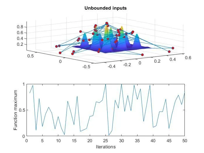
• The points were outside the search space and the Global Maxima was not obtained. Therfore this case was a failure.

Study -2:

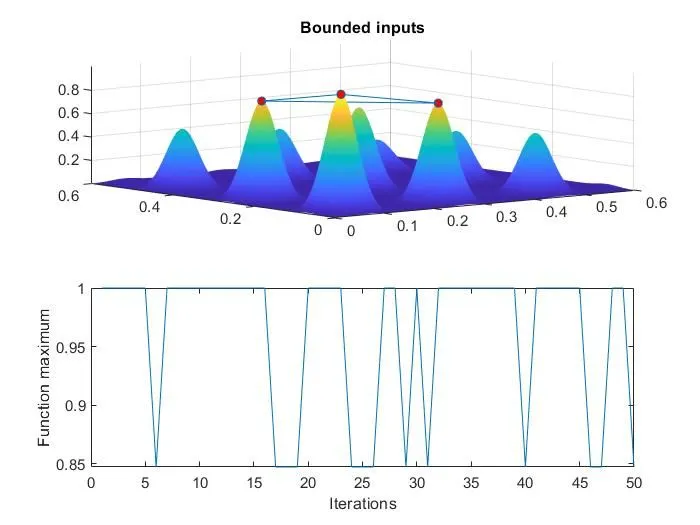
• Eventhough the plots were within the bounds ,the results were still far from the best but was better than study 1.

Study -3:

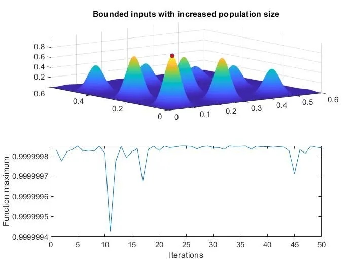
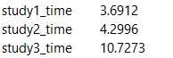
• As the population size(iterations) was increased, the evulation time was more but the Global Maxima was obtained. Therfore, this was the best result from the study cases.

CONCLUSION:

The stalagmite function was optimized and the Global Maxima was found.