Project 1 - Parsing NASA thermodynamic data

OBJECTIVE:

• To write code in MATLAB that extracts 14 co-efficients and calculates the enthalpy, entropy and Cp for all the species from the given data file (THERMO.dat).
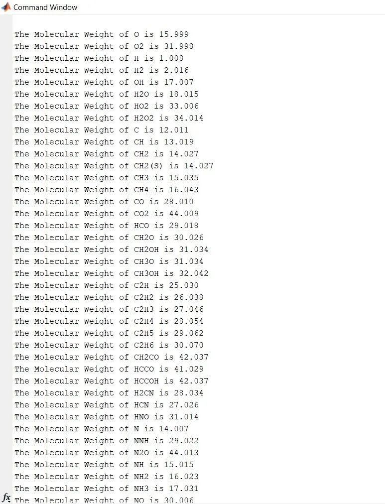
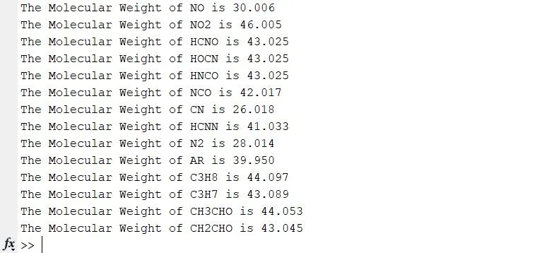
• To calculate the molecular weight of each species and display it in the command window.
• To plot the Cp, Enthalpy and Entropy for the local temperature range (low temperature : high temperature) specific for each species.
• To save the plots as images with appropriate names and dump them in separate folders for each species with suitable name. All these should be generated automatically.

FILE PARSING:

• To parse data or information means to break it down into component parts so that its syntax can be analyzed, categorized, and understood.
• NASA came up with polynomials that can be used to evaluate thermodynamic properties such as Cp, H and S. They have also documented the co-efficients that are required to evaluate these polynomials for 1000+ species.

THEORY:

• Thermodynamic data for individual species are necessary for performing equilibrium chemistry and finite-rate chemical kinetics calculations. These data typically provide the thermodynamic properties (enthalpy, entropy, and specific heat) of a species as a function of temperature.
• Thermodynamic Properties:

(1) Enthalpy:

Enthalpy is a property of a thermodynamic system, and is defined as the sum of the system's internal energy and the product of its pressure and volume.

(2) Entropy:

Entropy is a scientific concept, as well as a measurable physical property that is most commonly associated with a state of disorder, randomness, or uncertainty. The term and the concept are used in diverse fields, from classical thermodynamics, where it was first recognized, to the microscopic description of nature in statistical physics, and to the principles of information theory.

(3) Heat Capacity (Cp):

In a system, Cp is the amount of heat energy released or absorbed by a unit mass of the substance with the change in temperature at a constant pressure. In another words, under a constant pressure it is the heat energy transfer between a system and its surrounding. So, Cp represents the molar heat capacity, C when pressure is constant. The change in temperature will always cause a change in the enthalpy of the system.

• The NASA polynomials have the form:
  Cp/R = a1 + a2 T + a3 T^2 + a4 T^3 + a5 T^4
  
  H/RT = a1 + a2 T /2 + a3 T^2 /3 + a4 T^3 /4 + a5 T^4 /5 + a6/T
  
  S/R = a1 lnT + a2 T + a3 T^2 /2 + a4 T^3 /3 + a5 T^4 /4 + a7

where R is the Universal Gas Constant and ,a1, a2, a3, a4, a5, a6, and a7 are the numerical coefficients supplied in NASA thermodynamic files. The first 7 numbers starting on the second line of each species entry (five of the second line and the first two of the third line) are the seven coefficients (a1 through a7, respectively) for the high-temperature range. The following seven numbers are the coefficients (a8 through a14 in the program, respectively) for the low-temperature range.

CODE:

MAIN CODE:

clear all 
close all
clc

f = fopen('THERMO.dat','r')   % Opening a new file
line1 = fgetl(f);             

% Extracting the global temperatures
Global_temp_str = fgetl(f);   
G_Ts = strsplit(Global_temp_str,' ');
global_l_temp = str2num(G_Ts{2});  
global_m_temp = str2num(G_Ts{3});
global_h_temp = str2num(G_Ts{4});
cmmnt1 = fgetl(f); % comment
cmmnt2 = fgetl(f); % comment
cmmnt3 = fgetl(f); % comment

%Universal Gas Constant
R = 8.3145; % [J mol-1 k-1]

%% Species block
for i = 1:53                       % Starting a loop for each species

species_head = fgetl(f);    
sn = strsplit(species_head,' ');
species_name = (sn{1});              % Extracting the species name

% Extracting the local temperatures from the header line of the species
% block
loctemp_str = findstr(species_head,'.');
species_head(loctemp_str(1)-3:loctemp_str(1)+3);

local_l_temp = str2num(species_head(loctemp_str(1)-3:loctemp_str(1)+3));
local_h_temp = str2num(species_head(loctemp_str(2)-4:loctemp_str(2)+3));
local_m_temp = str2num(species_head(loctemp_str(3)-4:loctemp_str(3)+3));

temp = linspace(local_l_temp,local_h_temp,500);      % creating  low to high range  local temperature values

% Extracting the coefficients a1 to a5 from line-1 
species_line1 = fgetl(f);
L_1 = findstr(species_line1,'E');
a1 = str2num(species_line1(1:L_1(1)+3));
a2 = str2num(species_line1(L_1(1)+4:L_1(2)+3));
a3 = str2num(species_line1(L_1(2)+4:L_1(3)+3));
a4 = str2num(species_line1(L_1(3)+4:L_1(4)+3));
a5 = str2num(species_line1(L_1(4)+4:L_1(5)+3));

% Extracting the coefficients a6 to a10 from line-2

species_line2 = fgetl(f);
L_2 = findstr(species_line2,'E');
a6 = str2num(species_line2(1:L_2(1)+3));
a7 = str2num(species_line2(L_2(1)+4:L_2(2)+3));
a8 = str2num(species_line2(L_2(2)+4:L_2(3)+3));
a9 = str2num(species_line2(L_2(3)+4:L_2(4)+3));
a10 = str2num(species_line2(L_2(4)+4:L_2(5)+3));

% Extracting the coefficients a11 to a14 from line-3

species_line3 = fgetl(f);
L_3 = findstr(species_line3,'E');
a11 = str2num(species_line3(1:L_3(1)+3));
a12 = str2num(species_line3(L_3(1)+4:L_3(2)+3));
a13 = str2num(species_line3(L_3(2)+4:L_3(3)+3));
a14 = str2num(species_line3(L_3(3)+4:L_3(4)+3));


%Specific Heat Calculation
cp = specific_heat(a1,a2,a3,a4,a5,a8,a9,a10,a11,a12,R,temp,global_m_temp);

%Enthalpy Calculation
H = enthalpy(a1,a2,a3,a4,a5,a6,a8,a9,a10,a11,a12,a13,R,temp,global_m_temp);

%Entropy Calculation
S = entropy(a1,a2,a3,a4,a5,a7,a8,a9,a10,a11,a12,a14,R,temp,global_m_temp);

%------------------------- plot -----------------------------

% Specific Heat vs Temperature

figure(1)
plot(temp,cp,'linewidth',2,'color','b')
title(sprintf('Cp vs Temperature for %s',species_name))
xlabel('Temperature [K]')
ylabel('Cp [KJ/(mol K)]')
grid on

% Enthalpy vs Temperature

figure(2)
plot(temp,H,'linewidth',2,'color','r')
title(sprintf('Enthalpy vs Temperature for %s',species_name))
xlabel('Temperature [K]')
ylabel('Enthalpy[KJ/mol]')
grid on

% Entropy vs Temperature

figure(3)
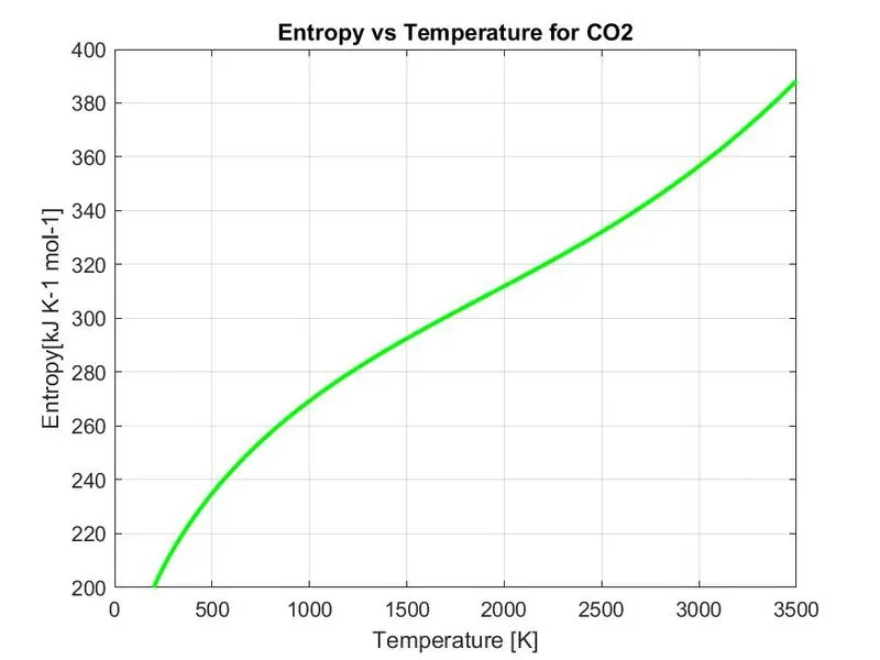
plot(temp,S,'linewidth',2,'color','g')
title(sprintf('Entropy vs Temperature for %s',species_name))
xlabel('Temperature [K]')
ylabel('Entropy[kJ K‑1 mol-1]')
grid on

% Making a new folder
directory = (['F:\Matlab pgms\MATLAB PROJECT 1\species_data\',species_name]);
mkdir(directory)

%saving the plots for each species in the created folder
cd(['F:\Matlab pgms\MATLAB PROJECT 1\species_data\',species_name])


saveas(figure(1),'Cp.jpg')
saveas(figure(2),'Enthalpy.jpg')
saveas(figure(3),'Entropy.jpg')
cd(['F:\Matlab pgms\MATLAB PROJECT 1']);

% Molecular Weight Calculation

m_w = molecular_weight(species_name);
disp(sprintf('The Molecular Weight of %s is %.3f ',species_name,m_w))



end

EXPLANATION:

1. The file 'THERMO.dat' is opened using fopen command.
2. The data is read line by line using the fgetl command.
3. Comments and other unimportant lines are ignored.
4. The global temperatures are extracted as seperate strings using strsplit command and converted to numbers using str2num command and is stored in different variables.
5. The Universal Gas Constant R is initiated.
6. A for loop is started to extract the coefficients for the 53 species.
7. Inside the loop, name of the species is read and assigned to a variable by using the strsplit command.
8. From the same line the local temperatures are extracted by using the strfind command.
9. Using the linspace command, 500 values are generated for the local temperature range(low to high).
10. Using the strfind command with 'E' as the delimitter, each coefficients from a1 to a14 is extracted from the three lines of the species block and is converted to number using the str2num command.
11. Three functions to calculate the Cp, Enthalpy and Entropy respectively is called.
12. The relation of the Cp, Enthalpy and Entropy with the local temperatures are plotted seperately
13. A new folder is created using the mkdir command and the three plots for each species are saved in seperate folders using cd and saveas command.
14. The function to calculate the molecular weight of each species is called.
15. The molecular weight of each species is displayed in the command window.

FUNCTION CODE TO CALCULATE CP:

function cp = specific_heat(a1,a2,a3,a4,a5,a8,a9,a10,a11,a12,R,temp,local_m_temp)

if temp >= local_m_temp  %For High temperature coefficients
    cp = R*(a1 + (a2*temp) + (a3*(temp.^2)) + (a4*(temp.^3)) +(a5*(temp.^4))); 
    
else  %For Low temperature coefficients
    cp = R*(a8 + (a9*temp) + (a10*(temp.^2)) + (a11*(temp.^3)) + (a12*(temp.^4)));

end

Cp = R*(a1 + a2 T + a3 T^2 + a4 T^3 + a5 T^4)

1. The input parameters given are the coefficients,R value, temperature range and the local medium temperature.
2. Using the formula given above, the Cp value for each species was calculated according to the temperature range with the help of if-else conditions.

FUNCTION CODE TO CALCULATE ENTHALPY:

function H = enthalpy(a1,a2,a3,a4,a5,a6,a8,a9,a10,a11,a12,a13,R,temp,local_m_temp)

if temp >= local_m_temp  %For High temperature coefficients
    H = R*temp.*(a1 + (a2.*temp) + ((a3.*(temp.^2))/2) + ((a4.*(temp.^3))/3) + ((a5.*(temp.^4))/4) + (a6./temp));
    
else %For Low temperature coefficients
    H = R*temp.*(a8 + (a9.*temp) + ((a10.*(temp.^2))/2) + ((a11.*(temp.^3))/3) + ((a12.*(temp.^4))/4) + (a13./temp));
    
end

H= R*T*(a1 + a2 T /2 + a3 T^2 /3 + a4 T^3 /4 + a5 T^4 /5 + a6/T)

1. The input parameters given are the coefficients,R value, temperature range and the local medium temperature.
2. Using the formula given above, the Enthalpy of each species was calculated according to the temperature range with the help of if-else conditions.

FUNCTION CODE TO CALCULATE ENTROPY:

function S = entropy(a1,a2,a3,a4,a5,a7,a8,a9,a10,a11,a12,a14,R,temp,local_m_temp)

if temp >= local_m_temp %For High temperature coefficients
    S = R.*((a1.*log(temp)) + (a2.*temp) + ((a3.*(temp.^2))/2) + ((a4.*(temp.^3))/3) + ((a5.*(temp.^4))/4) + a7);
else %For Low temperature coefficients
    S = R.*((a8.*log(temp)) + (a9.*temp) + ((a10.*(temp.^2))/2) + ((a11.*(temp.^3))/3) + ((a12.*(temp.^4))/4) + a14);


end

S =R* (a1 lnT + a2 T + a3 T^2 /2 + a4 T^3 /3 + a5 T^4 /4 + a7)

1. The input parameters given are the coefficients,R value, temperature range and the local medium temperature.
2. Using the formula given above, the Entropy of each species was calculated according to the temperature range with the help of if-else conditions.

FUNCTION CODE TO CALCULATE THE MOLECULAR WEIGHT:

function M = molecular_weight(species_name)
element = ['H','C','N','O','A'];

atom_w = [1.008,12.011,14.007,15.999,39.95];

M = 0;

for i = 1:length(species_name)
    for j = 1:length(element)
        if strcmp(species_name(i),element(j))
            M = M + atom_w(j);
            pos = j;
        end
    end
    num = str2num(species_name(i));
    if num>1
        M = M + atom_w(pos)*(num-1);
    end

end

1. The species name is given as the input parameter.
2. As each species is made up of chemical elements, a string array containing the required elements is initiated.
3. An array containing the Atomic Weight of the required elements is also initiated.
4. The molecular weight variable was initiated as 0.
5. With the help of nested for loop and the strcmp command to compare the species name with the elements, the Molecular weight was calculated.

OUTPUTS:

COMMAND WINDOW :

f =

    12

The Molecular Weight of O is 15.999 
The Molecular Weight of O2 is 31.998 
The Molecular Weight of H is 1.008 
The Molecular Weight of H2 is 2.016 
The Molecular Weight of OH is 17.007 
The Molecular Weight of H2O is 18.015 
The Molecular Weight of HO2 is 33.006 
The Molecular Weight of H2O2 is 34.014 
The Molecular Weight of C is 12.011 
The Molecular Weight of CH is 13.019 
The Molecular Weight of CH2 is 14.027 
The Molecular Weight of CH2(S) is 14.027 
The Molecular Weight of CH3 is 15.035 
The Molecular Weight of CH4 is 16.043 
The Molecular Weight of CO is 28.010 
The Molecular Weight of CO2 is 44.009 
The Molecular Weight of HCO is 29.018 
The Molecular Weight of CH2O is 30.026 
The Molecular Weight of CH2OH is 31.034 
The Molecular Weight of CH3O is 31.034 
The Molecular Weight of CH3OH is 32.042 
The Molecular Weight of C2H is 25.030 
The Molecular Weight of C2H2 is 26.038 
The Molecular Weight of C2H3 is 27.046 
The Molecular Weight of C2H4 is 28.054 
The Molecular Weight of C2H5 is 29.062 
The Molecular Weight of C2H6 is 30.070 
The Molecular Weight of CH2CO is 42.037 
The Molecular Weight of HCCO is 41.029 
The Molecular Weight of HCCOH is 42.037 
The Molecular Weight of H2CN is 28.034 
The Molecular Weight of HCN is 27.026 
The Molecular Weight of HNO is 31.014 
The Molecular Weight of N is 14.007 
The Molecular Weight of NNH is 29.022 
The Molecular Weight of N2O is 44.013 
The Molecular Weight of NH is 15.015 
The Molecular Weight of NH2 is 16.023 
The Molecular Weight of NH3 is 17.031 
The Molecular Weight of NO is 30.006 
The Molecular Weight of NO2 is 46.005 
The Molecular Weight of HCNO is 43.025 
The Molecular Weight of HOCN is 43.025 
The Molecular Weight of HNCO is 43.025 
The Molecular Weight of NCO is 42.017 
The Molecular Weight of CN is 26.018 
The Molecular Weight of HCNN is 41.033 
The Molecular Weight of N2 is 28.014 
The Molecular Weight of AR is 39.950 
The Molecular Weight of C3H8 is 44.097 
The Molecular Weight of C3H7 is 43.089 
The Molecular Weight of CH3CHO is 44.053 
The Molecular Weight of CH2CHO is 43.045 
>> 

PLOTS:

O2:

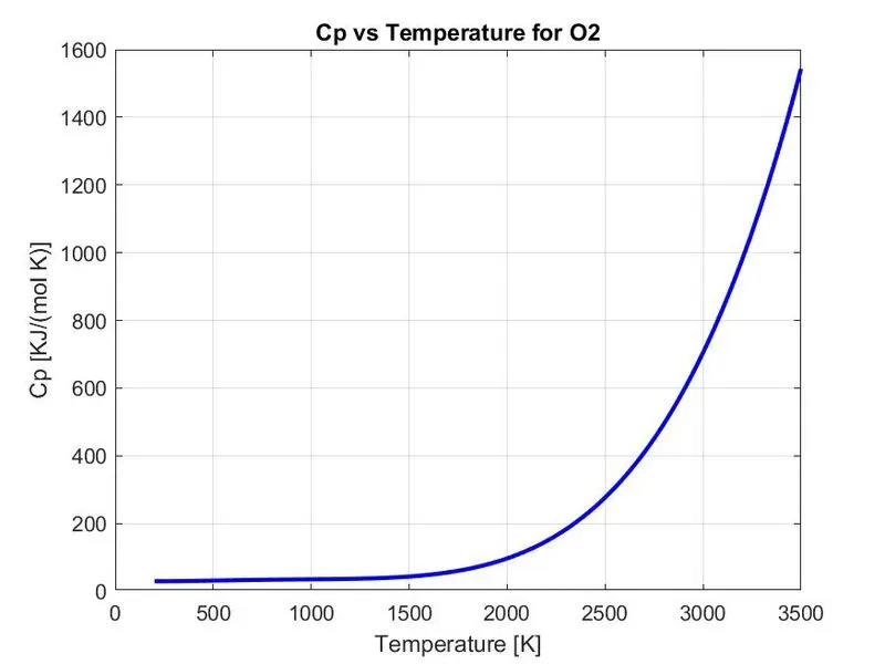
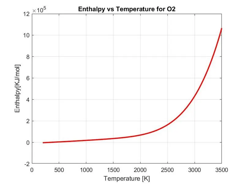
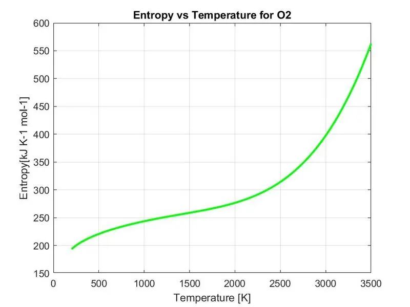
N2:

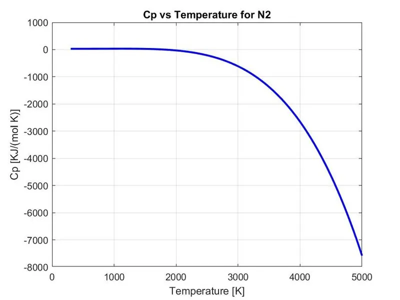
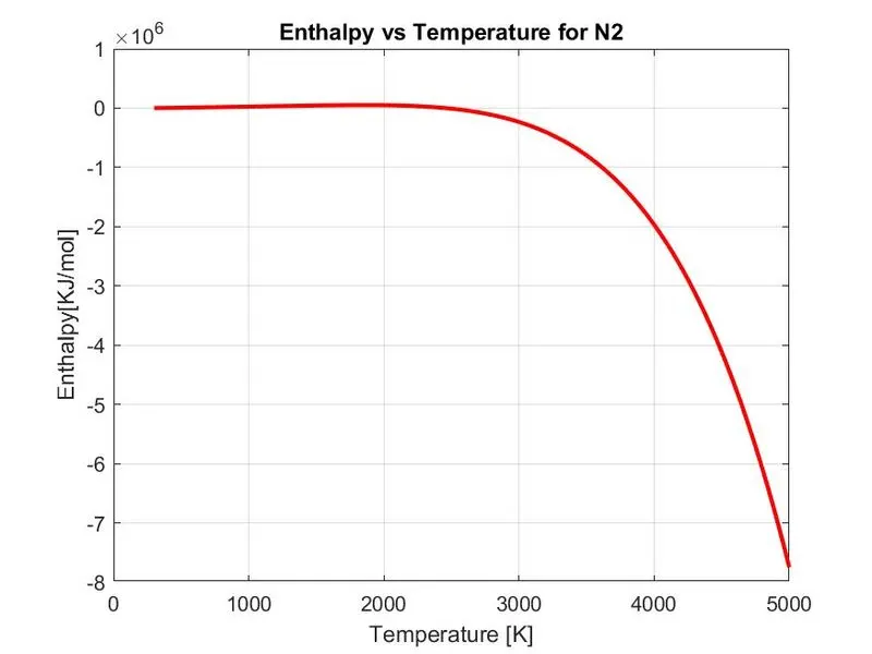
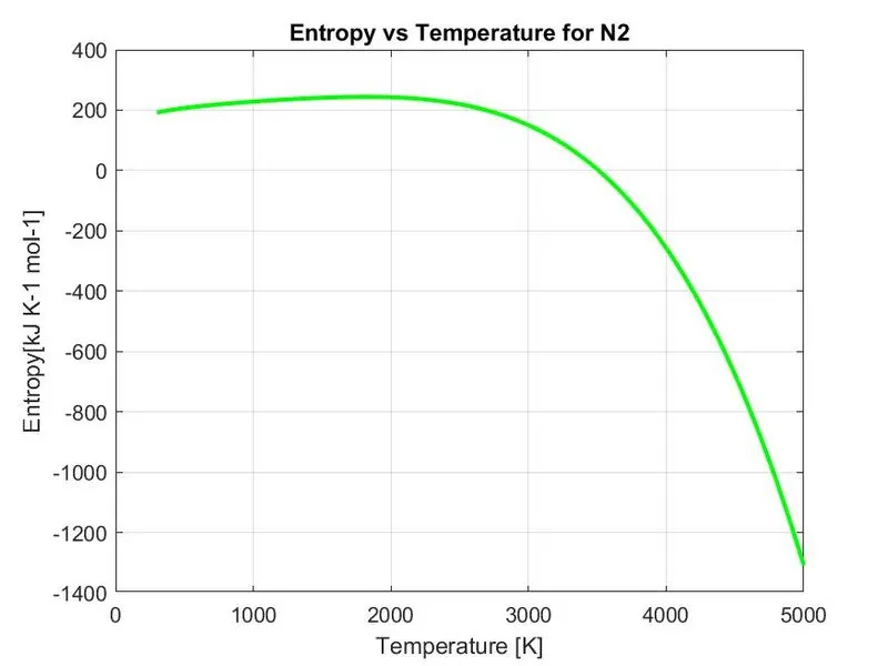
CO2:

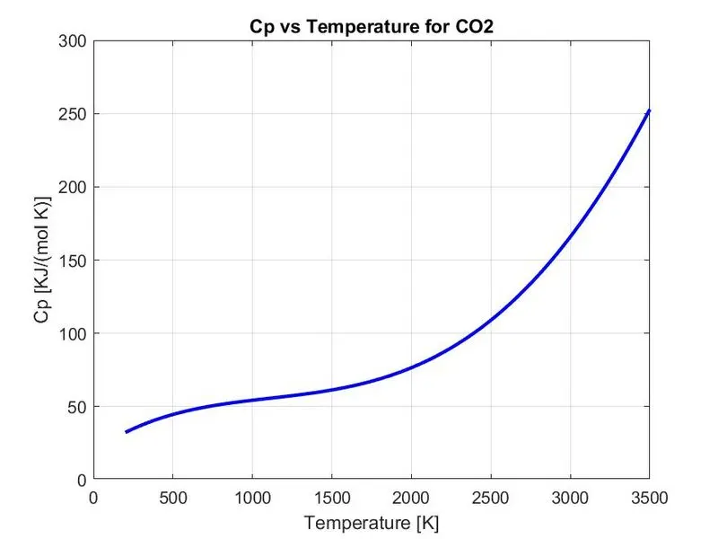
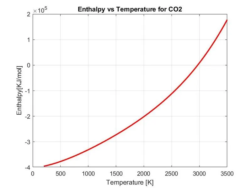
SPECIES DATA FOLDER SCREENSHOT:

COMMAND WINDOW SCREENSHOT:

CONCLUSION:

The 14 coefficients for each species was extracted from the data file. Their thermodynamic properties were calculated and plots were obtained.