Week 3 - Solving second order ODEs

OBJECTIVE:

• The write a program that solves the ODE which represents the equation of motion of a simple pendulum with damping and to animate the same using MATLAB.
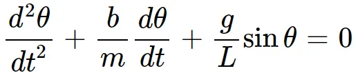
•  The ODE is:

                  `

EXPLANATION

• The following values were used for the ODE:

1.   Length of the pendulum(L) = 1 m
2. Mass of the ball(m) = 1 kg
3. Damping coefficient(b) = 0.05
4. Acceleration due to gravity(g) =9.81 m/s^2

•  In the code, the initial condition was taken as 0 for angular displacement and angular velocity 3 rad/sec at time t=0.
• Time span was also initialized using linspace function.
• The next step is to solve the equation using an in-built solver in MATLAb called ode45 where we define it as a function of t and theta. A function(ode_function) was defined inside the ode45 solver along with the initial condtions as parameters.
• The function ode_function takes t,theta,b,g,l,m as parameter and breaks the Second order ODE to two first order ODE and returns a solution vector.
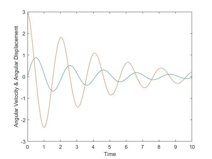
• After solving the equation using ode45, a time vs Angular Displacement and Angular velocity plot was created.

Then the code for animation was written.

• A variable ct for counting each frame was initiated as 1 and a for loop was started.
• The fixed starting points of the pendulum string was assigned as 0.
• The end of the string(where the bob is attached) was assigned as the sin and cos functions of the ODE solution.
• Then the plot was made for the fixed support and the string.
• The bob was plotted using marker command.
• Each plotted figure was captured using the 'getframe' function and and was assigned to another variable M and the count was incremented.
• A movie was created in 'avi' format and each captured frame was written inside the videofile and was saved.

RESULTS:

The ODE was solved and an animation was created out of it.

THE MAIN CODE:

% Second Order ODE
clear all
close all
clc

% Input,
b = 0.05;
g = 9.81;
l = 1;
m = 0.1;

% Initial Condition
theta_0 = [0;3];

% Time Points
t_span =  linspace(0,10,500);

% Solving the ODE

[t, results] = ode45(@(t,theta) ode_function(t,theta,b,g,l,m),t_span,theta_0);

% Plot

plot(t,results(:,1))
hold on
plot(t, results(:,2))
xlabel('Time')
ylabel('Angular Velocity & Angular Displacement')

% Animation for the pendulum

ct = 1;
for i = 1:length(results(:,1))
    x0 = 0;
    y0 = 0;
    x1 = l*sin(results(i,1));
    y1 = -(l*cos(results(i,1)));
    figure(2)
    plot([-1 1],[0 0],'linewidth',3,'color','r');
    hold on
    plot([x0 x1],[y0 y1],'linewidth',3,'color','b');
   
    plot(x1,y1,'o','markersize',25,'markerfacecolor','g','markeredgecolor','b');
    hold off
    grid on
    
    axis([-1 2 -1.5 0.5])
    pause(0.0000000001)
    M(ct) = getframe(gcf);
    ct = ct+1;
    
end

% Animation video creation
movie(M)
video = VideoWriter('Simple Pendulum.avi','Uncompressed AVI');
open(video)
writeVideo(video,M)
close(video)

THE FUNCTION CODE:

% function code to get the solution

function [dtheta_dt] = ode_function(t,theta,b,g,l,m)

theta1 = theta(1)
theta2 = theta(2)
dtheta1_dt = theta2;
dtheta2_dt = -(b/m)*theta2 - (g/l)*sin(theta1);
dtheta_dt = [dtheta1_dt; dtheta2_dt];




end

THE 'Time vs Angular displacement & Angular velocity' PLOT:

GOOGLE DRIVE LINK OF THE ANIMATION:

https://drive.google.com/file/d/1MwzhCnEsUVdeG6ZQDlUZRN9mB-DTtzC0/view?usp=sharing