Week 4.1 - Genetic Algorithm

Aim:

To write code to optimise the stalagmite function and find the global maxima of the function, using MATLAB.

Theory:

Genetic Algorithm (GA) is a randomized search algorithm and an optimization technique based on the principles of Genetics and Natural Selection. It is used to find optimal solutions to difficult problems. This algorithm reflects the process of natural selection where the fittest individuals are selected for reproduction in order to produce offspring of the next generation.

The process of natural selection starts with the selection of fittest individuals from a population. They produce offspring which inherit the characteristics of the parents and will be added to the next generation. If parents have better fitness, their offspring will be better than parents and have a better chance at surviving. This process keeps on iterating and at the end, a generation with the fittest individuals will be found.

The algorithm repeatedly modifies a population of individual solutions. At each step, the genetic algorithm randomly selects individuals from the current population and uses them as parents to produce the children for the next generation. Over successive generations, the population "evolves" toward an optimal solution.

Applications in Real World

Genetic algorithm has many applications in real world. Here I have listed some of the interesting application, but explaining each one of them will require me an extra article.

1. Engineering Design- Engineering design has relied heavily on computer modelling and simulation to make design cycle process fast and economical. Genetic algorithm has been used to optimize and provide a robust solution.
2. Traffic and Shipment Routing (Travelling Salesman Problem)-This is a famous problem and has been efficiently adopted by many sales-based companies as it is time saving and economical. This is also achieved using genetic algorithm.
3. Robotics-The use of genetic algorithm in the field of robotics is quite big. Actually, genetic algorithm is being used to create learning robots which will behave as a human and will do tasks like cooking our meal, do our laundry etc.

Steps Involved:

1. First, define the objective function which is Stalagmite function in our case.
2. Define inputs x and y using “linspace” command.
3. A 2D array is generated using “meshgrid” command to plot surface of the Function output.
4. Now obtain the output of Stalagmite Function at various inputs(x,y).
5. Now, calculate the maximum values of the stalagmite function for given inputs by using the genetic algorithm(ga) which is in-built function in MATLAB.
6. GA gives minimum value which in this case is used to get maxima by giving a Negative sign to the output of stalagmite function.
7. Surfc and Plot command is used to plot the results in three iterations which are “Unbounded Iterations”, “Bounded Iterations” and “Increasing Population Size”.

The Stalagmite Function is as follows:

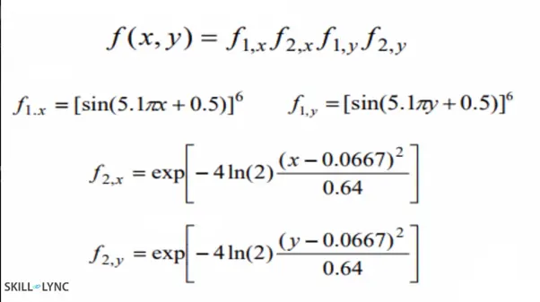
The Stalagmite Function is as follows:

function [f1] = stalagmite_func(input_vector)

f1x= [sin(((5.1*pi)*input_vector(1)) + 0.5)]^6 ;
f1y= [sin(((5.1*pi)*input_vector(2)) + 0.5)]^6 ;
f2x=exp((((input_vector(1)-0.0667).^2)/0.64).*(-4*log(2)));
f2y=exp((((input_vector(2)-0.0667).^2)/0.64).*(-4*log(2)));
f=f1x*f1y*f2x*f2y;
f1=-f;%the negative sign inverse the Stalagmite function output thus giving the global maxima
end

The syntax for ga is explained as below,

x - Minimum value that ga function returns

fun – the objective function which is maximized (Here it is stalagmite)

nvars - no. of design variables of the function

A,b - Linear Inequalities which the function is subjected to

Aeq,beq - Linear equalities which the function is subjected to

lb,ub - lower and upper bounds on the design variables

nonlcon- nonlinear constraints

options- to perform operations like increasing population size using “optimoptions”

The following code studies the Statistical behaviour under 3 conditions namely

1. Unbounded Inputs

2. With Lower and Upper Bounds

3. With Increased Population Size

clear all
close all
clc

x=linspace(0,0.6,150);
y=linspace(0,0.6,150);
num_cases=50;
[xx yy] = meshgrid(x,y);

%Evaluating the stalagmite function

for i=1: length(xx)
    for j= 1: length(yy)
        input_vector(1)=xx(i,j);
        input_vector(2)=yy(i,j);
        f(i,j)=stalagmite_func(input_vector);
    end
end

%Study 1 - Statistical Behaviour for Unbounded Inputs
tic
for i=1:num_cases
    [inputs,fopt(i)]=ga(@stalagmite_func,2);
    xopt(i)=inputs(1);
    yopt(i)=inputs(2);
end
study_time1=toc

%Plotting the graph
figure(1)
subplot(2,1,1)
hold on
surfc(x,y,f);
shading interp
plot3(xopt,yopt,fopt);
title('Unbounded Inputs')
subplot(2,1,2)
plot(fopt)
xlabel('Iterations')
ylabel('Functions Minimum')

%Study 2 - Statistical Behaviour for Bounded Inputs
tic
for i=1:num_cases
    [inputs,fopt(i)]=ga(@stalagmite_func,2,[],[],[],[],[0;0],[1;1]);
    %A, B, Aeq and Beq = [] as linear inequalities and equalities does not
    %exist in this function
    %lower boundary is set at [0;0] and upper boundary at [1;1];
    xopt(i)=inputs(1);
    yopt(i)=inputs(2);
end
study_time2=toc

%Plotting the graph
figure(2)
subplot(2,1,1)
hold on
surfc(x,y,f);
shading interp
plot3(xopt,yopt,fopt);
title('Bounded Inputs')
subplot(2,1,2)
plot(fopt)
xlabel('Iterations')
ylabel('Functions Minimum')

%Study 3 - Statistical Behaviour by defining a population size
%Defining the population size
options= optimoptions('ga')
options=optimoptions(options,'PopulationSize',170);

tic
for i=1:num_cases
    [inputs,fopt(i)]=ga(@stalagmite_func,2,[],[],[],[],[0;0],[1;1],[],[],options);
    %A, B, Aeq and Beq = [] as linear inequalities and equalities does not
    %exist in this function
    %lower boundary is set at [0;0] and upper boundary at [1;1];
    %options help defin the population size in the algorithm
    xopt(i)=inputs(1);
    yopt(i)=inputs(2);
end
study_time3=toc

%Plotting the graph
figure(3)
subplot(2,1,1)
hold on
surfc(x,y,f);
shading interp
plot3(xopt,yopt,fopt);
title('Inputs')
subplot(2,1,2)
plot(fopt)
xlabel('Iterations')
ylabel('Functions Minimum')

Results and Conclusion:

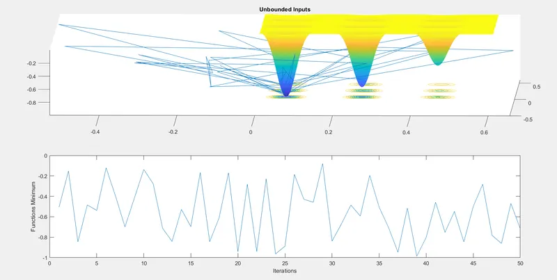
1. Plot obtained for Unbounded Inputs

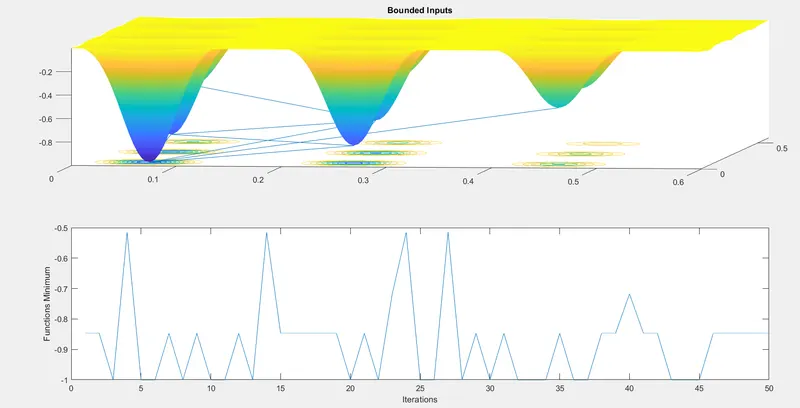
2. Plot obtained for running GA with Boudned Inputs

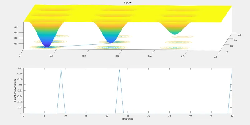
3. Plot obtained for running GA with Increased Population Size

The study time for each studies are respectively

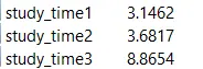
Thus we see that with more population, GA takes more time to reach to optimum solution.

From above we can conclude that GA works more efficiently with bounded limits and with increased no. of Polpulation Size and iterations.

It can also be seen that GA does not run within the search space defined as seen in the first study. It is only when Bounded inputs are given, we can reach to satisfactory results.

References:

1. https://towardsdatascience.com/introduction-to-genetic-algorithms-including-example-code-e396e98d8bf3

2. https://www.analyticsvidhya.com/blog/2017/07/introduction-to-genetic-algorithm/

3. https://www.tutorialspoint.com/genetic_algorithms/genetic_algorithms_introduction.htm

4. https://www.sciencedirect.com/topics/engineering/genetic-algorithm

5. https://in.mathworks.com/discovery/genetic-algorithm.html