Week 3 - Solving second order ODEs

Aim: To solve the ODE of Simple Pendulum Motion and animate the simulation of a pendulum using Matlab.

Theory: A Simple pendulum consist of a bob or a point mass attached to a string(of neglible mass) suspended to a fixed point. In ideal conditions, it follows a SHM i.e. when given a small displacement from its mean position(or equilibrium position), a restoring force(here its weight i.e. mgsinθ">θ) accelerates the bob in the opposite direction of its initial displacement i.e. towards the mean position. At extreme position, its potential energy gets converted to kinetic energy which gives it sufficient velocity to return to its mean postion. But at equilibrium all its potential energy is being converted to kinetic energy and thus have maximum velocity which further displaces the bob from its mean position but this time in opposite direction and can be easily understood as shown below.

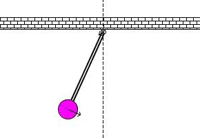
The forces acting on pendulum in case of ideal conditions is shown below

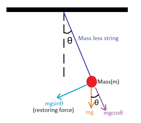
Now, this motion is only in ideal conditions where we neglect the effect of air drag(i.e. air friction). in case of air drag which acts as dampling force the velocity reduces if not given constant force and this motion can be represented by the following equation which is derived using Newton's 2nd law,

`(d^2theta)/dt^2 + (b/m)(d theta)/dt + (g/l)sintheta = 0`

where,

g = gravity in m/s2,

L = length of the pendulum in m,

m = mass of the ball in kg,

b=damping coefficient.

Now, in order to solve the ODE in MATLAB we first break it into two single order equations,

let `theta=theta1`

`(dθ)/dt=(dθ1)/dt=θ2`

Inserting the values of `theta=theta1` and `(d theta)/dt=theta2` in equation (1) we get,

`(dθ2)/dt + b/mθ2 + g/lsinθ1=0`

thus two ODEs θ">θ2(displacement) and `(dθ2)/dt`(velocity)

`d/dt[[theta1],[theta2]]=[[theta2],[-b/mtheta2-g/lsintheta1]]`

The code to solve the ODE

clear all
close all
clc

%inputs
b=0.05; %damping coefficient
g=9.81; %acceleration due to gravity
l=1; %length of massless string
m=1; %mass of bob

%initial conditions
theta_0 =[0;3];

%time points
t_span=linspace(0,20,200);

%solve ode
[t,results]= ode45(@(t,theta) ode_func(t,theta,b,g,l,m), t_span, theta_0);

%plotting
plot(t,results(:,1),'linewidth',1,'color','r')
hold on
plot(t,results(:,2),'linewidth',1,'color','b')
legend('Displacement','Velocity')
xlabel('Time')
ylabel('Plot')

Explainantion:

1. We use 'clear all', 'close all' and 'clc' to clear inputs, workspace and command window of previous programs.

2. The inputs are then assigned to variables and initial condition is assigned to variable theta_0(initial dispacement is 0 as it is displaced from its mean position and 3 is initial velocity).

3. t_span is the limits between 0 and 20 seconds for which the motion is being studied.

4. we use a function ode45 which is inbuilt ODE solver in Matlab, its syntax is

[t,y]=ode45(odefun,tspan,y`theta`)

where tspan = [t0 tf], integrates the system of differential equations y′=f(t,y) from t0 to tf with initial conditions y0. Each row in the solution array y corresponds to a value returned in column vector t.

Function:

function [dtheta_dt]= ode_func(t,theta,b,g,l,m)

theta1=theta(1);
theta2=theta(2);
dtheta1_dt=theta2;
dtheta2_dt=-(b/m)*theta2- (g/l)*sin(theta1);
dtheta_dt=[dtheta1_dt; dtheta2_dt];
end

Result:

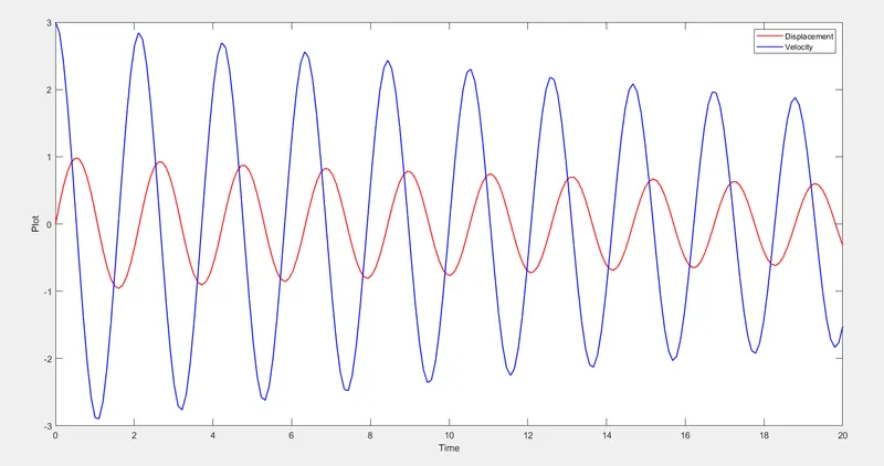
Now for animation,

The Program is as below,

clear all
close all
clc

b=0.05;
g=9.81;
l=1;
m=1;

%initial conditions
theta_0 =[0;3];

%time points
t_span=linspace(0,20,200);

%solve ode
[t,results]= ode45(@(t,theta) ode_func(t,theta,b,g,l,m), t_span, theta_0);

ct=1;
O=[0,0];

for i=1:length(t) %i will run for the time span t i.e. the pendulum time span
    p=-l*sin(results(i,1)); %p is x-axis coordinate at angle returned at i respectively
    q=-l*cos(results(i,1)); %q is y-axis coordinate at angle returned at i respectively
    plot([O(1) p],[O(2) q],'marker','o') %to plot the two points between (0,0) and (p,q)
    axis([-3 2 -3 2])
    pause(0.01)
    M(ct)=getframe(gcf);
    ct=ct+1;
end

movie(M)
videofile=VideoWriter('ode_challenge.avi', 'Uncompressed AVI');
open(videofile)
writeVideo(videofile,M)
close(videofile)

Explaination:

1. p & q is X and Y coordinate for the other point at theta obtained from results.

2. i runs for t time value.

3. p is the point at l*sinθ length from (0,0) on left side(which is signified by '-' sign)

4. q is the point at l*cosθ length from (0,0) below( which is signified by '-' sign)

Result:

https://drive.google.com/file/d/1NiOIYRcw3iW866__kOh7_Ouw18PNWwWk/view?usp=sharing