Week 4.1 - Genetic Algorithm

AIM: To study about genetic algorithm and to calculate the global maxima of stagalmite function using Genetic algorithm in MATLAB

OBJECTIVE:

• To write a code in MATLAB to optimise the stalagmite function and find the global maxima of the function.
• To expalin the concept of genetic algorithm and also explain the syntax for ga in MATLAB in the report.
• Plot graphs for all 3 studies and for F maximum vs no. of iterations. Title and axes labels are a must, legends could be shown.

THEORY:

CONCEPT OF GENETIC ALGORITHM:

A genetic algorithm (GA) is a method for solving both constrained and unconstrained optimization problems based on a natural selection process that mimics biological evolution. The algorithm repeatedly modifies a population of individual solutions. At each step, the genetic algorithm randomly selects individuals from the current population and uses them as parents to produce the children for the next generation. Over successive generations, the population "evolves" toward an optimal solution.

STALAGMITE FUNCTION:

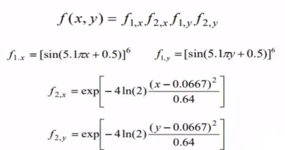
A stalagmite function generally refers to the function with which we are generating values over a stalagmite kind of surface for finding out the local and global maxima and minima of that particular given function.

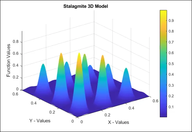
The stagalmite function is given as follows:

EXPLANATION OF CODE:

• Firstly we create our own function to calculate the value of objective function at variables x and y.
• We use linspace command to create x and y values.
• Now we create a matrix using meshgrid function.
• We created the values in different matrices and put in the function,then we get the function values of x and y.
• For our case1,we will use the for loop and iterate it 50 times.
• We will use the following syntax

[inputs,fopt]=ga(function,no of variables)

Here the no of variables are 2 that is x and y,the inputs1*2 matrix for each iteration,it will basically x and y and fopt will give the optimum function at these x and y values.

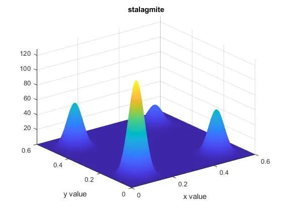
We can use the surf command to create a 3D visualisation and we can also use the marker command to find the points of local maximum.

Tictac command is used to look at the time taken for evaluation.

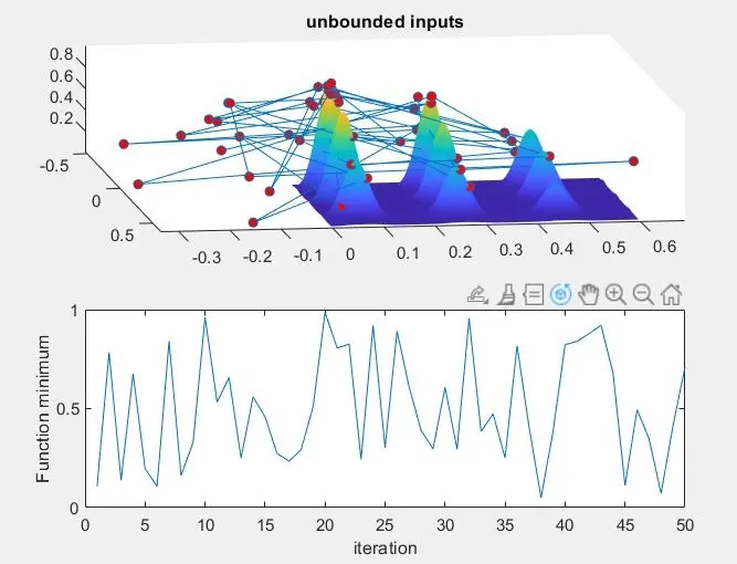
The results of case1 is that ga command doesn't know the bound of these x and y values.

Hence we setup the upper and lower boundsm fo9r this ga function and the syntax is:

[inputs,fopt]=ga(function,no of variables,a,b,aeq,beq,lb,ub) where

lb is lower bound and ub is upper bound

a-linear inequality constraints

b-linear inequality constraints

aeq-linear equality connstraints

beq-linear equality connstraints

a,b,aeq,beq represented as empty array,hence the syntax is

[inputs,fopt]=ga(function,no of variables,[],[],[],[],lb,ub)

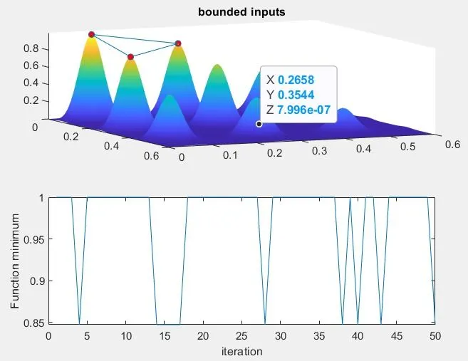
If we execute the loop we will get different local maximas with bounded inputs,still it is not showing correct local maximas,then we need to increase the population size to converge a global maximum.The syntax is

[inputs,fopt]=ga(function,no of variables,[],[],[],[],lb,ub,[],[],options).

GENETIC ALGORITHM CODE:

close all
clear all
clc
%inputs
x=linspace(0,0.6,150);
y=linspace(0,0.6,150);

%matrices
[xx yy]=meshgrid(x,y);
% no of iterations
num_values=50;

for i=1:length(xx)
    for j=1:length(yy)
        input_vector(1)=xx(i,j);
        input_vector(2)=yy(i,j);
        f(i,j)=stalagmite_function(input_vector);
    end    
end
%creates the three dimensional surface
figure(1);
surfc(xx,yy,-f);
shading interp
xlabel('x value');
ylabel('y value');
title('stalagmite');

%case1 with unbounded inputs
tic
for i=1:num_values
    [inputs,fopt(i)]=ga(@stalagmite,2);
    xopt(i)=inputs(1);
    yopt(i)=inputs(2);
end
case_1=toc
figure(2);
subplot(2,1,1);
surfc(x,y,-f);
hold on;
xlabel('x value');
ylabel('y value');
title('unbounded inputs');

shading interp

plot3(xopt,yopt,-fopt,'marker','.','markersize',5,'markerfacecolor','r');
subplot(2,1,2);
plot(-fopt);
xlabel('iterations');
ylabel('function maximum');

%case2 with upper and lower bounds
tic
for i=1:num_values
    [inputs,fopt(i)]=ga(@stalagmite,2,[],[],[],[],[0;0],[0.6,0.6]);
    xopt(i)=inputs(1);
    yopt(i)=inputs(2);
end
case_2=toc
figure(3);
subplot(2,1,1);
hold on;
surfc(x,y,-f);
xlabel('x value');
ylabel('y value');
title('bounded inputs');

shading interp

plot3(xopt,yopt-fopt,'marker','.','markersize',5,'markerfacecolor','r');
subplot(2,1,2);
plot(-fopt);
xlabel('iterations');
ylabel('function maximum');

%case_3 increasing the population size

tic
for i=1:num_values
    [inputs,fopt(i)]=ga(@stalagmite,2,[],[],[],[],[0;0],[0.6,0.6],[],[],opt);
    xopt(i)=inputs(1);
    yopt(i)=inputs(2);
end
case_3=toc
figure(4);
subplot(2,1,1);
hold on;
surfc(x,y,-f);
xlabel('x value');
ylabel('y value');
title('bounded inputs with increased population size');

shading interp

plot3(xopt,yopt-fopt,'marker','.','markersize',5,'markerfacecolor','r');
subplot(2,1,2);
plot(-fopt);
xlabel('iterations');
ylabel('function maximum');

THE FUNCTION CODE:

function [f]=stalagmite_function(input_vector)
a=input_vector(1);
b=input_vector(2);

term1=((sin(5.1*pi*a)+0.5))^6;
term2=exp(-4*log(2)*((a-0.0667)^2)/0.64);
term3=((sin(5.1*pi*b)+0.5))^6;
term4=exp(-4*log(2)*((b-0.0667)^2)/0.64);
[f]=-(term1*term2*term3*term4);
end