Week 3 - Solving second order ODEs

AIM: To solve an ordrinay differential equation(ODE) and use the calculated information to animate the motion of the pendulum.

INTRODUCTION:

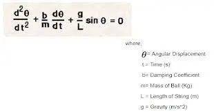
In engineering,ODE is used to describe the transient behaviour of the system.A eg is simple pendulum.The following is the second order ODE of a simple pendulum.The way the pendulum moves depends on the newton second law.

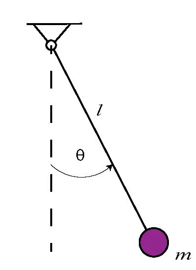
FORMULAE:

CODE:

%function for solving ODE
function [dtheta_dt]=ode_function(t,theta,b,g,l,m)
theta1=theta(1);
theta2=theta(2);
dtheta1_dt=theta2;
dtheta2_dt=-(b/m)*theta2-(g/l)*sin(theta1);
[dtheta_dt]=[dtheta1_dt;dtheta2_dt]
end

close all
clear all
clc
%inputs
b=0.05;
g=9.81;
l=1;
m=0.5;
%initial conditions
theta_0=[0;5];

%time
t_span=linspace(0,20,500);
%solve ode
[t,results]=ode45(@(t,theta)ode_function(t,theta,b,g,l,m),t_span,theta_0);
figure(1);
plot(t,results(:,1));
hold on;

plot(t,results(:,2));
xlabel('time(sec)');
ylabel('position and angular velocity');
title('motion of the simple pendulum');
legend('Angular displacement','Angular velocity');

%To animate the pendulum
ct=1;
for i=1:length(results(:,1))
    x0=0;
    y0=0;
    x1=l*sin(results(i,1));
    y1=-l*cos(results(i,1));
    figure(2);
    plot([-0.5 0.5],[0 0],'linewidth',2);
     hold on;
    plot([x0 x1],[y0 y1],'linewidth',2,'color','r');
   
    plot(x1,y1,'marker','.','markersize',25);

    axis([-1.5 1.5 -2 2]);
    grid on;
    pause(0.03);
    M(ct)=getframe(gcf)
    ct=ct+1;
    hold off;
end
movie(M)
videofile=VideoWriter('damping_pendulum.avi','uncompressed avi');
open(videofile)
writeVideo(videofile,M)
close(videofile)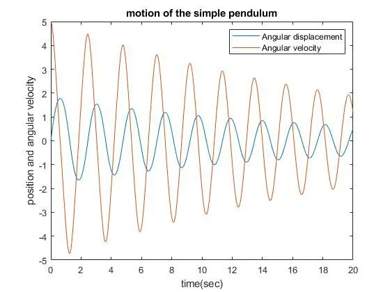

The animation of the pendulum link below:

https://youtu.be/qUv0-nnpiVg