Week 4.1 - Genetic Algorithm

Problem Statement:

• Write a code in MATLAB to optimize the stalagmite function and find the global maxima of the function.
• Clearly explain the concept of genetic algorithm in your own words and also explain the syntax for ga in MATLAB in your report.
• Make sure that your code gives the same output, even if it is made to run several times.
• Plot graphs for all 3 studies and for F maximum vs no. of iterations. Title and axes labels are a must, legends could be shown if necessary

Solution:

Theory:

Genetic Algorithm:

• Genetic algorithm is an optimization tool in Matlab that is used to find the minimum value of a function.
• It is based on the evolution process in which the eligible candidates are selected, then these fit candidates are allowed to cross and produce fitter candidates belonging to the next generation. Then these candidates undergo mutation during their lifetime in the generation. And so on the process repeats to following generations.
• A genetic algorithm works with the fitness function. This function evaluates the fitness of the individuals. Fitness function defines the eligibility criteria for selection of the fruitful candidates.
• At the beginning, initial population is recruited. Without specification, the initial population is randomly selected. As this process is unrestricted, the population consists of the points out of the boundary and outside the scope of the function under consideration.
• These points are run through the fitness function in order to select the better candidates. In this case, the points, which create the local maxima are selected.
• Then these points are allowed to cross over. The point which returns the lowest value for the defined function has better chances of bequeathing its genes to the descending generation. Hence, the set of points that minimize the function, are allowed to cross over and produce the next generation of points.
• The new set of points undergo mutation. Here, the genes are interchanged to tranform into the slightly better candidates. This set becomes the initial population for the upcoming generation and the process is repeated for 100 generation by default.
• syntax for genetic algorithm in Matlab:
  • [x, fval] = ga(fun,nvars,A,b,[],[],lb,ub,nonlcon,IntCon,options)
  • x is an array which stores the points generated by ga at which local and global minima can be found.
  • fval stores the local and global minima
  • fun- fitness function that the points need to satisfy
  • nvars- number of variables that serve as input arguments to fitness function
  • A,b - inequality constraints
  • lb-Lower bond or the minimum value of the points
  • ub-upper bond or the maximum value of points
  • options- structure datatype variable that helps the ga with populationsize, etc

Procedure to define the fitness function:

1. Use the function command to define the function. Store the output in 'f'
2. Accept the output in array form in which x values are stored in 1st column and y values are stored in 2nd column
3. Define the various terms in stalagmite function and multiple to get output 'f'
4. Since GA is the minimization tool, it finds the minimum value of the function. Hence the function is negated to obtain maximum value.

Code:

%Defining the stalagmite function
function f=stalagmite(inp)

f1x=(sin(5.1*pi*inp(1)+0.5))^6;
f1y=(sin(5.1*pi*inp(2)+0.5))^6;
f2x=exp(-4*log(2)*(inp(1)-0.0667)^2/0.64);
f2y=exp(-4*log(2)*(inp(2)-0.0667)^2/0.64);

%Negating the function value to obtain maxima instead of minima
f=-(f1x*f1y*f2x*f2y);

end

Procedure for obtaining stalagmite function values:

1. get_stalagmite function accepts the x and y values as input
2. Use meshgrid command to generate mesh of x and y
3. Use for loop to run through the whole mesh and access the all the defined gridpoints
4. The x and y value at every grid point is passed to stalagmite function and function value is obtained

Code:

%Function to generate meshgrid and obtain the stalagmite values
function f=get_stalagmite(x,y)
[xx yy]=meshgrid(x,y);
for i=1:length(xx)
    for j=1:length(yy)
        input_vector(1)=xx(i,j);
        input_vector(2)=yy(i,j);
        f(i,j)=stalagmite(input_vector);
    end
end

Procedure for running Genetic Algorithm to obtain global maxima:

1. Generate the equispaced values on x and y axis using linspace command.
2. Use the values as input to get_stalagmite function to obtain the stalagmite values at all grid points.
3. In the first study, only the fitness function and number of variables are passed as input in 'ga' function. Hence this study case is unbounded in nature.
4. All the fit coordinates are stored in inputs and segregated into xout and yout variables. fout stores the global and local maxima.
5. The results are plotted. 'srfc' command is used to plot contours under the surface plot. 'shading' command is used to remove the grid lines on the surface and 'interp' command is used for interpolation, to smoothen the curve. 'plot3' command is used to plot the values in 3-dimensions. The results obtained from 'ga' is used to mark the coordinates in the 3D space which represent the global and local maxima. Then 'plot' command is used to plot the optimized function values againts every iteration. 'Subplot' command is used to divide the figure window to it in various plots. In this case, figure window is divided into 2 rows and 1 column.
6. In the second study, the lower bounds and upper bounds are also passed as input arguments in 'ga'. lb=[0 0] which stores the lowest limits of both x and y. And ub=[0.6 0.6] which stores the greatest limit of both x and y.
7. Since there are no linear inequalities, empty matrices [] are passed in the corresponding position within 'ga'.
8. Similarly, the same plots are generated with better results.
9. In the third study, the population size is defined additionally. 'Options' is of structure data type, which is used to create populationsize of 170. Whenever the input variables for fitness function is 2, then the population size is set to 50 by default. This value is increased to obtain better output.
10. Again the similar plots are generated.

Code:

clear all
close all
clc

%Creating the points for stalagmite funtion
x=linspace(0,0.6,150);
y=linspace(0,0.6,150);

%Obtaining stalagmite function values at all defined points
f=get_stalagmite(x,y);

%Number of times to run the ga function to study the variance
num_cases=50;

%Study 1: Unbounded condition 
for i=1:num_cases
    [inputs,fout(i)]=ga(@stalagmite,2);
    xout(i)=inputs(1);
    yout(i)=inputs(2);
end
%Plotting resultant values from ga
figure (1)
subplot(2,1,1);
hold on
surfc(x,y,f);
shading interp
plot3(xout,yout,fout,'marker','o');
subplot(2,1,2);
plot(fout);
xlabel('Iteration')
ylabel('Optimized fuction value')



%Study 2: Bounded condition with defined upper and lower bonds 
for i=1:num_cases
    [inputs,fout(i)]=ga(@stalagmite,2,[],[],[],[],[0;0],[0.6;0.6]);
    xout(i)=inputs(1);
    yout(i)=inputs(2);
end
%Plotting the result in figure 2
figure (2)
subplot(2,1,1);
hold on
surfc(x,y,f);
shading interp
plot3(xout,yout,fout,'marker','o');
subplot(2,1,2);
plot(fout);
xlabel('Iteration')
ylabel('Optimized fuction value')

%study 3: Bounded contion with defining the population size
options=optimoptions('ga');
options=optimoptions(options,'populationsize',170);

for i=1:num_cases
    [inputs,fout(i)]=ga(@stalagmite,2,[],[],[],[],[0;0],[0.6;0.6],[],[],options);
    xout(i)=inputs(1);
    yout(i)=inputs(2);
end
%Plotting the results in figure 3
figure (3)
subplot(2,1,1);
hold on
surfc(x,y,f);
shading interp
plot3(xout,yout,fout,'marker','o');
subplot(2,1,2);
plot(fout);
xlabel('Iteration')
ylabel('Optimized fuction value')

Errors:

1. 
   • In this error, the input_vector array was directly stored in x (input argument) of stalagmite function. So x was treated as an array. The issue was resolved by definining stalgamite with array 'inp' as input arguments and then indexing was used to segregate x and y values.
2. 
   1. Global optimization toolbox was missing and hence 'ga' function was not performed. This was resolved by downloading the toolbox.
3. 
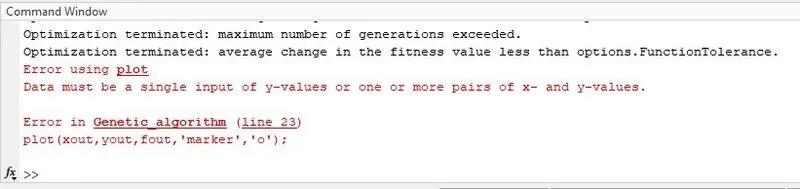
   • 'plot' command was used to plot 3-D data. This was resolved by using 'plot3' command instead.

Output:

1. 
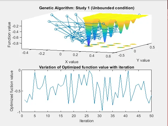
   • In the unbounded condition, it can be seen that the population is randomly selected in the space. Hence the points obtained are out of the scope of the stalagmite function. And the maximum function value is very erratic and lies in the range of 0 and -1.
2. 
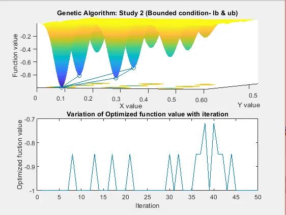
   • In the restricted condition, the obtained points lie in the scope of the stalagmite function. The range of the maximized function value also shrinks to be limited between -0.7 and -1.
3. 
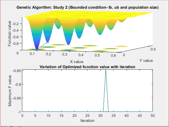
   • In this study, the population size is defined. Thus the optimized function value range is further shrunk. The genetic algorithm narrows the maxima of stalagmite to only 2 peaks as seen in the plot.