Project 2 - Rankine cycle Simulator

Problem statement:

• Create a Rankine Cycle Simulator using OCTAVE/MATLAB.
• Your code should calculate the state points of the Rankine Cycle (any type of your choice) based on user inputs.
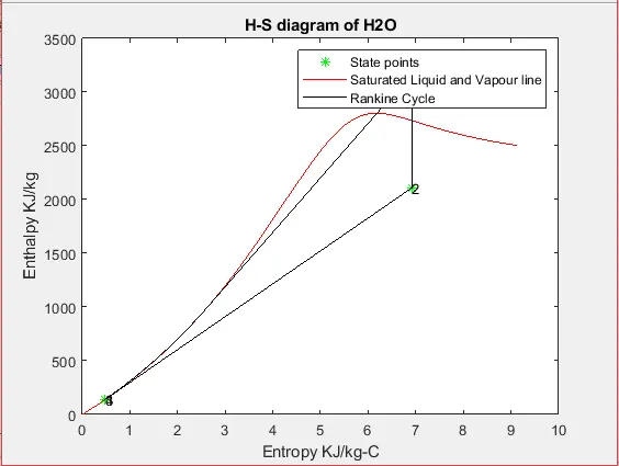
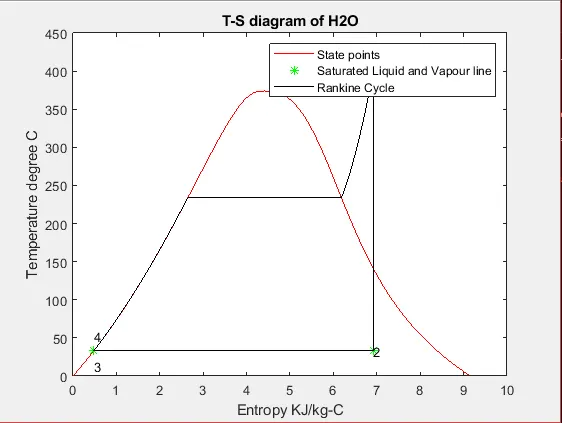
• Then, plot the corresponding T-s and h-s plots for the given set of inputs. Title and axes labels are a must, while legends could be used if necessary.
• The presentation of your code will be taken into consideration while grading. Labelling sections of your code using comments is appreciated.
• Attach a report explaining the working of a Rankine cycle simulator and also the research done by you.

Theory:

The Rankine cycle is a thermodynamic cycle that is used in powerplants to produce useful mechanical work by expanding the superheated water in the turbine. The steps in the Rankine cycle are as follows:

1-2: Isentropic Expansion: In this process, the superheated steam is expanded in the turbine. The turbine blades rotate and produce useful work Wt. During this process, the entropy of water remains the same:s1=s2. Due to expansion, the pressure p1 and temperature T1 reduce to p2 and T2. Enthalpy also drops to H2 from H1. The expansion process is hindered by the cooling temperature range of the condenser and by the erosion of the turbine blades. Due to this, the dryness fraction of the exiting steam should be well over 90%.

2-3: Isobaric Heat Rejection: In this process, the turbine exiting steam is passed through the condenser. Within this device, the phase transformation of the water to liquid takes place. As the pressure is constant, P2=P3. Enthalpy drops to h3 due to loss of heat and entropy also reduces to s3. The cooling medium is generally seawater, which absorbs the heat of the steam and is discarded back to the ocean.

3-4: Isentropic Compression: In this process, the liquid water is pressurized in the pump, hence the pressure increases to p4. While entropy remains constant, hence s3=s4. Enthalpy increases in this process to h4. Here, the work done Wp is negative, since the energy is supplied to the pump.

4-1: Isobaric Heat Addition: In this process, the high-pressure liquid water enters the boiler. At the exit of the boiler, the water is superheated to a temperature T1. Pressure remains the same during this process, hence p4=p1. Enthalpy and entropy increase by the maximum amount to h1 and s1.

The work done by the turbine is given by Wt=h1-h2.

The work done by the pump is given by Wp= h4-h3.

Back Work Ratio: It is the fraction of work done by the turbine which is absorbed by the pump. bwr=Wp/Wt

Procedure:

1. Display the steps of the Rankine cycle in the command window using disp() and fprintf() commands.
2. Create three prompts to get the inputs from the user using input() and store the corresponding input in the appropriate state point variable. The working fluid is at state point 1 at the inlet of the turbine. Hence store inlet temperature in T1, inlet pressure in p1 and exit pressure in p2.
3. Using XSteam() function, obtain the enthalpy, entropy and temperature of the saturation vapour. XSteam() takes the name of the data seeked and the corresponding state point values as input arguments. In the first argument, V stands for saturated vapour, L for saturated liquid, h for enthalpy and so on.
4. Use if condition to check if the water superheated or saturated vapour at inlet of turbine.
   1. If water is superheated, obtain enthalpy and entropy at point 1 using XSteam() as a function of pressure and temperature.
   2. If water is saturated vapour, then enthalpy and entropy will be equal to previously obtained values.
5. At state point 2, entropy remains unchanged.
6. In order to calculate the dryness fraction, first obtain the values of entropy of saturated liquid and vapour at pressure p2 using XSteam() and substitute in the formula.
7. Obtain the values of enthalpy and temperature of saturated vapour at pressure p2.
8. Check for the dryness fraction to calculate the state point 2 values.
   
   1. If x2=1, then it is saturated vapour. In this case state point 2 properties are equal to properties at saturated vapour line at p2.
   2. If x2<1, then the water is mixture of liquid and vapour. In this case, obtain enthalpy value by supplying pressure p2 and dryness fraction value. T2 will be same as saturation temperature at p2.
   3. If x2>1, the water is still superheated steam. T2 and h2 values are obtained by using XSteam() for p2 and s2 values.
9. At state point 3, pressure at this point remains the same.
10. T3,s3,h3 values are obtained for saturated liquid at pressure p3.
11. At state point 4, entropy remains the same. And pressure increases back to p1 level, as ideal Rankine cycle is reversible. T4 and h4 values are obtained by using function of p4 and s4 values.
12. Net work done and back work ratio are calculated by substituting the enthalpy values.
13. Then data for the diagram is prepared. Temperature values are created from 0 deg Celcius to critical temperature using linspace(). For all the values of temperature, enthalpy and entropy values are obtained for saturated liquid phase and stored in arrays.
14. Temperature values in array are reversed using fliplr(). Then again, corresponding enthalpy and entropy values are obtained from XSteam() for saturated vapour phase..
15. Entropy array is created from s4 to s1 for 4-1 process. And respective enthalpy and temperature values are obtained at pressure p1 and sequential entropy data.
16. Again, entropy array is created from s2 to s3 for process 2-3. And respective enthalpy and temperature values are obtained at pressure p2 and sequential entropy data.
17. Using figure command, two different figures are created for T-S and H-S diagram.
18. Plot command is used to plot the diagrams for saturated water first and then for rankine cycle. Legend is used to symbolize the various markers and line. Text command is used to mark all the points on the plot.
19. The results are printed on the command window using disp() and fprintf() function.

Code:

clear all
close all
clc

%Displaying the steps in the Rankine cycle
fprintf("ttttRankine Cycle Simulator:nn");
disp("1-2 is Isentropic Expansion process in the Turbine");
disp("2-3 is Constant Pressure Heat Rejection Process in the Condenser");
disp("3-4 is Isentropic Compression Process in the Pump");
disp("4-1 is Constant Pressure Heat Addition Process in the Boiler");

%Seeking the inputs from the user 
prompt1="nEnter the turbine inlet temperature: ";
T1=input(prompt1);
prompt2="Enter the turbine inlet pressure: ";
p1=input(prompt2);
prompt3="Enter the turbine exit pressure: ";
p2=input(prompt3);

%State point 1 calculation
hg1=XSteam('hV_p',p1);
sg1=XSteam('sV_p',p1);
Tsat1=XSteam('TSat_p',p1);
%Checking whether the steam at turbine inlet is superheated or saturated vapour
if T1>Tsat1
      h1=XSteam('h_pT',p1,T1);
      s1=XSteam('s_pT',p1,T1);
else if T1==Tsat1
        h1=hg1;
        s1=sg1;
     end
end

%State point 2 calculation
s2=s1;
sf2=XSteam('sL_p',p2);
sg2=XSteam('sV_p',p2);
%Calculating the dryness fraction
x2=(s2-sf2)/(sg2-sf2);
hg2=XSteam('hV_p',p2);
hf2=XSteam('hL_p',p2);
Tsat2=XSteam('TSat_p',p2);
%Checking if the steam at the turbine outlet is superheated, saturated
%vapour or mixture of vapour and liquid.
if x2==1 % Steam is saturated vapour
    h2=hg2;
    s2=sg2;
    T2=Tsat2;
else if x2<1 %Steam is mixture 
        h2=XSteam('h_px',p2,x2);
        T2=Tsat2;
    else  %Steam is superheated 
        T2=XSteam('T_ps',p2,s2); 
        h2=XSteam('h_ps',p2,s2);
        
    end
end

% State point 3 calculation:
p3=p2; %Isobaric process, so pressure remains same.
h3=XSteam('hL_p',p3);
s3=XSteam('sL_p',p3);
T3=XSteam('Tsat_p',p3);

%State point 4 calculation:
p4=p1; 
s4=s3; 
h4=XSteam('h_ps',p4,s4);
T4=XSteam('T_ps',p4,s4);

net_work=(h1-h2)-(h4-h3);
bwr=(h4-h3)/(h1-h2); %Back Work Ratio

%Preparing data for T-S and H-S diagram of water 
Tc=373.9457; %Critical temperature of water in deg Celcius
T_L=linspace(0,Tc,500); %Temperature range for saturated liquid line
for i=1:length(T_L)
    STL(i)=XSteam('sL_T',T_L(i));
    HTL(i)=XSteam('hL_T',T_L(i));
end
T_V=fliplr(T_L); % Temperature range for saturated vapour line
for i=1:length(T_V)
    STV(i)=XSteam('sV_T',T_V(i));
    HTV(i)=XSteam('hV_T',T_V(i));
end

%Data for process 4-1 of Rankine cycle
s41=linspace(s4,s1,500);
for i=1:length(s41)
    T41(i)=XSteam('T_ps',p1,s41(i));
    h41(i)=XSteam('h_ps',p1,s41(i));
end

%Data for process 1-2 of Rankine Cycle
s23=linspace(s2,s3,500);
for i=1:length(s23)
    T23(i)=XSteam('T_ps',p2,s23(i));
    h23(i)=XSteam('h_ps',p2,s23(i));
end

%Plotting T-S diagram of water and Rankine cycle
figure(1)
plot([STL STV],[T_L T_V],'color','r');
hold on
%Marking the Temperature and entropy state points on the diagram
plot([s1,s2,s3,s4],[T1,T2,T3,T4],'*','color','g');
text([s1,s2,s3,s4],[T1,T2,T3-20,T4+20],{'1','2','3','4'});
plot([s41,s23],[T41,T23],'color','k')
xlabel('Entropy KJ/kg-C');
ylabel('Temperature degree C');
title('T-S diagram of H2O');
legend('State points','Saturated Liquid and Vapour line','Rankine Cycle');

%Plotting H-S diagram of water and Rankine cycle:
figure(2)
%Marking the Enthalpy and Entropy State points on the diagram
plot([s1,s2,s3,s4],[h1,h2,h3,h4],'*','color','g');
hold on
%Numbering the state points
text([s1,s2,s3,s4],[h1,h2,h3,h4],{'1','2','3','4'});
plot([STL STV],[HTL HTV],'color','r');
plot([s41 s23],[h41 h23],'color','k');
legend('State points','Saturated Liquid and Vapour line','Rankine Cycle');
xlabel('Entropy KJ/kg-C');
ylabel('Enthalpy KJ/kg');
title('H-S diagram of H2O');




fprintf("ntttttResultsnn");
disp("At State point 1:");
fprintf("P1 is : %f Barn",p1);
fprintf("T1 is : %f deg Celciusn",T1);
fprintf("H1 is : %f KJ/kgn",h1);
fprintf("S1 is : %f KJ/kg-deg Celciusnn",s1);
disp("At State point 2:");
fprintf("P2 is : %f Barn",p2);
fprintf("T2 is : %f deg Celciusn",T2);
fprintf("H2 is : %f KJ/kgn",h2);
fprintf("S2 is : %f KJ/kg-deg Celciusnn",s2);
disp("At State point 3:");
fprintf("P3 is : %f Barn",p3);
fprintf("T3 is : %f deg Celciusn",T3);
fprintf("H3 is : %f KJ/kgn",h3);
fprintf("S3 is : %f KJ/kg-deg Celciusnn",s3);
disp("At State point 4:");
fprintf("P4 is : %f Barn",p4);
fprintf("T4 is : %f deg Celciusn",T4);
fprintf("H4 is : %f KJ/kgn",h4);
fprintf("S4 is : %f KJ/kg-deg Celciusnn",s4);
fprintf("Net workdone is : %f KJ/kgn",net_work);
fprintf("Back work ratio is : %f",bwr);


    

Output:

The result is attached in the pdf format.