Week 3 - Solving second order ODEs

Problem Statement:

Write a program in Matlab\Octave that will simulate the pendulum motion with the following parameters:

L=1 metre,

m=1 kg,

b=0.05.

g=9.81 m/s2.

Simulate the motion between 0-20 sec, for angular displacement=0,angular velocity=3 rad/sec at time t=0.

Theory:

The above given equation represents the second order ODE of a simple pendulum with damping. It is converted into first order ODE to obtain angular displacement and angular velocity as result.

Procedure:

1. ode_func function is created with input arguments
2. The equations are written as per the solved ODE
3. t_span is a row vector having values from 0 to 20 with 300 divisions. It represents the time instant at which the position of the pendulum is sought.
4. ode45 solver is used to solve the first order ODE with input parameters as
   1. Function definition: Here, the anonymous function is declared with t, theta as input arguments and the output of ode_func as the fuction definition.
   2. Time integral: Here, the time limits are specified over which ODE is integrated, that is the period from 0s to 20s
   3. Initial conditions: theta0 stores the initial angular displacement and velocity.
5. figure(1) is used to create first figure displaying angular velocity and displacement with respect to time. Hence the plot is used with input parameters as time t and results with all rows and 1st column since it holds the values of theta. Second plot command draws angular velocity stored in the 2nd column of results.
6. figure(2) displays the instantaneous position of the pendulum in an iterative manner. In every iteration, frame array M stores all the figures in series. 'hold on' command is used to hold all the plots of an iteration intact.
7. 'MarkerSize' command is used within plot to define the size of 'o' marker with 20.
8. 'movie' command is used to animate the series of figures

Code:

%function to obtain instantaneous angular displacent and angular velocity
function [dtheta_dt]=ode_func(b,g,l,m,t,theta)
% Represents the solved equation 
theta1=theta(1);
theta2=theta(2);

dtheta1_dt=theta2;
dtheta2_dt=-(b/m)*theta2-(g/l)*sin(theta1);

dtheta_dt=[dtheta1_dt;dtheta2_dt];
end

clear all
close all
clc

%input
b=0.05 
g=9.81
l=1
m=1

% Time span represented on the X-axis
t_span=linspace(0,20,300); 
% Initial conditions of the pendulum within a column vector
% Given data: velocity=3 rad/s and theta=0 rad at t=0 s
theta0=[0;3];
% Using the ode45 solver to obtain intantaneous position of the pendulum
[t,results]=ode45(@(t,theta) ode_func(b,g,l,m,t,theta),t_span,theta0);

% Plot of velocity and angular displacemnt against time
figure (1)
plot(t,results(:,1));
hold on
plot(t,results(:,2));
xlabel('Time');
ylabel('Plot');
hold off

% The point(x0,y0) representing the fixed end of the string
x0=0;
y0=0;

% For loop to obtain the instantaneous value of angular displacement
% To find the position of pendulum
for i=1:length(results) 
    theta_d=results(i,1); %Instantaneous angular displacement extracted from results
    y1=-l*cos(theta_d);% Vertical distance of pendulum from fixed support
    x1=l*sin(theta_d); % Horizontal distance of pendulum from fixed support
    figure (2) % Plot oscillatory movement of pendulum
    plot(x0,y0,'*')% Represents the fixed end of string
    hold on
    plot([-5 5],[0 0],'color', 'k') % Fixed support
    plot(x1,y1,'o','MarkerSize',20) % Represents the sphere of mass 1kg
    plot([x0 x1],[y0 y1],'linewidth',2) % String of the pendulum
    axis([-1.2 1.2 -1.5 0.2])
    k(i)=getframe(gcf) % Capturing the instantaneous frame of figure into array 'k'
    hold off %Switching the hold command to over-write new pendulum position
   
end

% Generating animation from the captured frames
movie(k);
videofile=VideoWriter('pendulum_motion.avi','Uncompressed AVI');
open(videofile);
writeVideo(videofile,k);
close(videofile);

Error:

Error encountered while running the code:

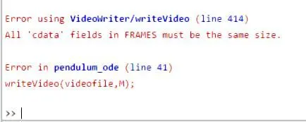
This was solved by changing the frame array name from 'M' to 'K'

Output:

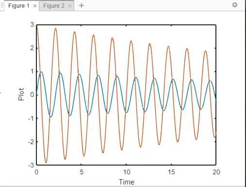
The output plot represents the change of angular displacement and velocity against the time span of 20s. As it can be seen, the initial velocity is 3 rad/s and displacement is 0 rad. As the damping coefficient has a low value, the pendulum motion takes a long time to dampen out. Due to damping, extreme position of the pendulum continues to decrease while the velocity at the mean position also continues to decrease.

Youtube link of the animation:

https://youtu.be/BpI8o90XZfc