P-V Diagram and Thermal Efficiency of Air Standard Otto Cycle using MATLAB

Aim:

To write code that can solve an otto cycle and make plot for it.

• Code creates a PV diagram
• Code outputs the thermal efficiency of the engine.

Theory:

The Otto Cycle is used to characterize the operation of the Spark Ignition Internal Combustion Engine. It was proposed by Nicholas Otto in 1876. It is considered to be the Air-Standard cycle with the following assumptions:

• Working fluid is air
• Air is treated as an ideal gas
• The combustion process is described by the heat addition process
• A heat rejection process is used to restore the system back to the original state
• All processes are internally reversible
• Constant and variable specific heats can be used

Otto cycle consists of four processes:

1-2: Isentropic compression process

2-3: Constant volume heat addition process

3-4: Isentropic expansion process

4-1: Constant volume heat rejection process

• Initially, at state point 1, properties of the system are Pressure- p1, Volume- v1, Temperature- t1. As the piston is at the Bottom Dead Centre (BDC), v1 is the same as the sum of clearance and swept volume, while pressure and temperature are the lowest.
• During 1-2 process, the entropy is constant and the piston starts moving away from the crankshaft, hence compressing the gas present in the cylinder above the piston. The system attains state point 2 when the piston reaches the Top Dead Centre (TDC). The properties of the system change to p2, v2, t2. p2>p1 and t2>t1, as due to compression, the pressure and temperature of the working fluid increase significantly according to the ideal gas equation: `p*v^gamma=constant` and `t*v^(gamma-1)`
• During 2-3 process, the volume is constant and heat is added to the system due to the combustion process. Pressure and temperature further increases to p3 and t3 according to the equation: `p/t=constant`
• During 3-4 process, entropy is constant and the piston moves towards the crankshaft and reaches BDC. As the result, the gas in the combustion chamber expands, thus expanding the volume to v4 (same as v1). The process reduces the pressure and temperature to p4 and t4.
• During 4-1 process, the volume is constant and the system rejects heat restoring it to the original state point (v1, p1, t1)

Engine Specification:

• Bore: Diameter of the cylinder in m
• Stroke: Distance travelled by the piston from BDC to TDC in m, which is also twice the length of crankpin
• Clearance volume: Volume of cylinder available on the top of the piston when it is located at TDC
• Swept volume: Volume of cylinder available when the piston is located at BDC
• Compression ratio: Ratio of cylinder volume at BDC and cylinder volume at TDC

Procedure:

1. The function is created to factor in the engine kinematic and consider the variation of pressure and volume at multiple instances of the crank angle. The function output is stored in 'v'
2. Crankpin length is calculated to obtain 'R' in the volume formula :
3. 'theta' angle is an array of 100 values ranging from start_crank angle to end_crank angle
4. Output 'v' is defined as the above-mentioned formula. The dot operator is used with 'theta', since it is a row vector.
5. In the main function, input variables are assigned such as bore, stroke, connecting rod length. Compression ratio (cr) is taken as 6 since it ranges from 6 to 10 for Spark-ignition engine. Gamma is taken as 1.4, as the air-standard cycle is assumed.
6. Initial pressure and temperature are taken as atmospheric pressure (1 Bar) and room temperature (300k). Maximum engine temperature is given.
7. State points for the otto cycle is obtained by ideal gas equation.
8. The curves for isentropic compression and expansion is obtained by calling the 'engine_kinematics' function with passing the input parameters. During the actual ICE operation: the crank angle (180 to 360 degrees) describe the compression process and the crank angle (360 to 540 degrees) describe the expansion process. Hence these angles are passed as an input argument for start_crank angle and end_crank angle to the function.
9. The incremental volume data against the crank angle obtained from the fuction is used to obtain incremental pressure data for the compression and expansion processes through the ideal gas equation.
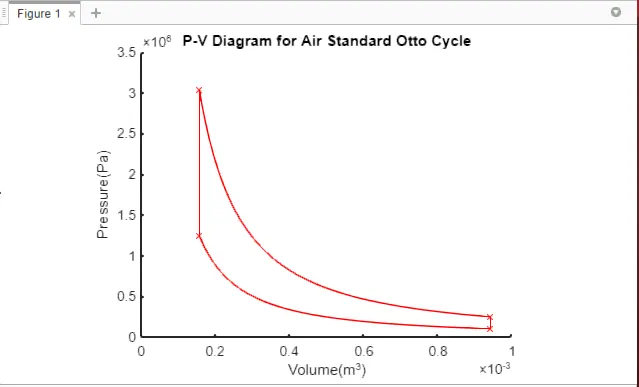
10. The state points are plotted on the P-V diagram using the 'plot' command with the marker '*' parameter. Curves are obtained for isentropic compression and expansion processes using 'plot' and straight lines are used to connect the state point 2-3 and 4-1.
11. 'title' command is used to entitle the figure and 'hold on' command is to plot multiple times on a single figure.

Code:

engine_kinematics function:

function V=engine_kinematics(bore,stroke,c_rod,cr,start_crank,end_crank)

crank_pin=stroke/2
R=c_rod/crank_pin
v_swept=(pi/4)*bore^2*stroke;
v_clearance=v_swept/(cr-1);

theta=linspace(start_crank,end_crank,100);

term1=0.5*(cr-1);
term2=R+1-cosd(theta)
term3=(R^2-sind(theta).^2).^0.5

V=(1+term1*(term2-term3))*v_clearance

end

Main function:

clear all
close all
clc

%Engine specifications
bore=0.1
stroke=0.1
c_rod=0.15
cr=6
gamma=1.4

%input
p1=101325
t1=300
t3=1500

%volume
v_swept=(pi/4)*bore^2*stroke
v_clearance=v_swept/(cr-1) %cr=(v_swept+v_clearance)/v_clearance

%state variables for the isentropic compression process
v1=v_swept+v_clearance
v2=v_clearance
p2= p1*cr^gamma %p1v1^gamma=p2v2^gamma-->p2=p1(v1/v2)^gamma
t2=p2*v2*t1/(p1*v1)

%curve for the isentropic compression process 
v_compression=engine_kinematics(bore,stroke,c_rod,cr,180,360);
const=p1*v1^gamma;
p_compression=const./v_compression.^gamma;

%state variables for constant volume heat addition process 
p3= p2*t3/t2 % p2/t2=p3/t3
v3=v2

%state variables for isentropic expansion process
v4=v1
p4=p3*(v3/v4)^gamma %p3v3^gamma=p4v4^gamma
t4=p4*v4*t3/(p3*v3)

%curve for isentropic expansion process
v_expansion=engine_kinematics(bore,stroke,c_rod,cr,360,540);
const=p3*v3^gamma;
p_expansion=const./v_expansion.^gamma;

figure(1)
hold on
plot(v1,p1,'*','color','r')
plot(v2,p2,'*','color','r')
plot(v_compression,p_compression,'Color','r')
plot(v3,p3,'*','color','r')
plot([v2 v3],[p2 p3],'color','r')
plot(v4,p4,'*','color','r')
plot(v_expansion,p_expansion,'Color','r')
plot([v4 v1],[p4 p1],'Color','r')
title('P-V Diagram for Air Standard Otto Cycle')
xlabel('Volume(m^3)')
ylabel('Pressure(Pa)')


%Calculating the thermal efficiency of otto cycle
n_thermal=1-1/cr^(gamma-1)

Result:

Diagram obtained from the code:

Thermal efficiency and state points obtained from the workspace as result:

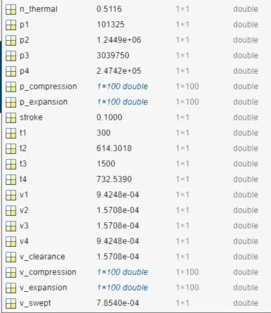
Thermal efficiency is 51.16%.