Week 4.1 - Genetic Algorithm
WRITING A CODE TO OPTIMISE THE STALAGMITE FUNCTION AND FIND THE OPTIMUM VALUE OF THE FUNCTION.
CONTENTS:
- EXPLANATION OF GENETIC ALGORITHM.
- SYNTAX OF GENETIC ALGORITHM.
- CASE1.
- PROGRAM1.
- OUTPUT1.
- CASE2.
- PROGRAM2.
- OUTPUT2.
- CASE3.
- OUTPUT3.
- PROGRAM3.
- ERRORS.
- RESULT.
- CONCLUSION.
EXPLANATION OF GENETIC ALGORITHM:
In computer science and operations research a genetic algorithm (GA) is a metaheurustic inspired by the process of natural selection that belongs to the larger class of evolutionary algorithms. Genetic algorithms are commonly used to generate highquality solutions to optimization and search problems by relyong on biologically isnipred operators such as mutation, crossover and selection. GA search parallel from a population of points. Therefore, it has the ability to avoid being trapped of points. Therefore, it has the ability to avoid being trapped in local optimal solution like traditional methods, which search from a single point. GA use prbablistic selection rules, not deterministic ones.This algorithm reflects the process of natural selection where the fittest individuals are seleceted for reproduction in order to produce offsprings of the next generation. Five phases are considered in a genetic alorithm they are as follows,
Intial population:
The process begins with a set of individuals, which is called a Population. Each individual is a solution to the problem you want to solve.
Fitness Function:
The Fitness function determines how fit an individual is to compete with the other individuals.The probability that an individual will be selected for reproduction is based on its fitness score.
Selection:
The idea of selection phase is to select the fittest individuals and let them pass their genes to the nesxt generation.Two pairs of individuals are selected based on their fitness score. Individuals with high fitness have more chance to be selected for reproduction.
Crossover:
Crossover is the most significant phase in a genetic algorithm.For each pair of parents to be mated, a crossover point is chosen at random from within the genes.Offsprings are created by exchanging the genes of parents among themselves until the crossover point is reached.
Mutation:
In certain new offspring formed, some of their genes can be subjected to a mutation with a low random probability. This implies that some of the bits in the bit string can be flipped.Mutation occurs to maintain diversity within the population and prevent premature convergence.
Termination:
The algorithm terminates if the population does not produce offsprings which are significantly different from the previous generation. Then it is said that genetic algorithm has provided a set of solutions to our problem.
THE SYNTAX FOR GA:
There are various syntaxs available in matlab for the function 'ga' but for this exercise alone i have described the syntaxs used in this program.
x=ga(fun,nvars)
x=ga(fun,nvars,A,B,Aeq,beq,lb,ub)
x=ga(fun,nvars,A,B,Aeq,beq,lb,ub,nonlcon,Intcon,options)
here,
'x' is the variable which stores the minimum value of the objective function.
'fun' is a fitness function.A fitness function is the function that takes a sampling solution and analyzes it for the output.
'nvars' is for the number of design variables we have given to it.
'A' and 'b' are used to represent the linear inequalities of the function if any.
'Aeq' and 'beq' are used to represent the equality constraints.
'lb' and 'ub' are used to specify the upper and lower bounds of the variables of the function.
'nonlcon' is a function that is specified using a function handle. A separate function code must be written as per the constraints of the function.
'Intcon' is used to specify the Integer constraint suc that the value of the function is an Integer.
'options' is used to provide the values of the default parameters using the named parameters, if the necessary of replacing the default parameters arises then it is done by using function of optimoptions.
CASE1-PROGRAM FOR OPTIMIZING THE STALAGMITE FUNCTION.
PROGRAM1:
clear all % used to clear the variables in the workspace
close all %used  to close all the figure windows
clc %used to clear the command window

%defining our search space by giving variables within our desired range
x= linspace(0,0.6,150);
y= linspace(0,0.6,150);

cases=50; %this is the number of iterations you want the genetic algorithm to run

%creating a two dimensional mesh
[xx yy]=meshgrid(x,y);

%Evaluating the stalgamite function

for i=1:length(xx)
%it shows the number of times you want the loop to run in this case from 1 to length of the 'xx' array.

for j=1:length(yy)
%it shows the number of times you want the loop to run in this case from 1 to length of the 'yy' array.

input_vector(1)=xx(i,j);
input_vector(2)=yy(i,j);
%here each time the loop runs the value of 'xx' and 'yy' is taken and input into variables respectively.

f(i,j)=stalagmite(input_vector);% here we are calling the stalagmite function with the values of 'xx' and 'yy'
end
end % end of for loop

%statistical behavior

tic % stopwatch timer starts

for i=1:cases %here the loop runs from 1 to till the defined number of cases.
[inputs,fopt(i)]=ga(@stalagmite,2);
%here function is called with '@' and 'ga' which is a inbuilt solver in matlab is used to solve the stalagmite function with the inputs we have provided.And the outputs will be saved in 2 arrays ' inputs' and fopt(i).

xopt(i)=inputs(1);
yopt(i)=inputs(2);
%here the optimal values of inputs are stored in 'xopt' and 'yopt' for every iteration of the loop.

end %end of loop
case_time=toc %time taken by the loop to calculate optimal values is calculated and output is given with the variable'case_time'

%plotting according to the genetic algorithm statistical behavior

subplot(2,1,1)%subplot is used to create more than one graph in the same window with 2 columns and 1 row.
hold on % hold or retain the plot
surfc(x,y,-f)% used to create 3 dimensional subplot.
shading interp % used for the smootheness of the surface.
plot3(xopt,yopt,-fopt,'marker','o','markersize',5,'markerfacecolor','red')% is used to create the optimal 'x' and 'y' and function values in the 3-D plot
xlabel('x')
ylabel('y')
zlabel('f')
%for labling of 'x','y' and 'f'.
subplot(2,1,2)
plot(-fopt,'color','b')%plotting to observe the variation with respectto optimal function value.
title('Unbounded Inputs')%title for the graph.
xlabel('Number of iterations')%x axis labling.
ylabel('Function Maxima')%y axis labling.
OUTPUT1:
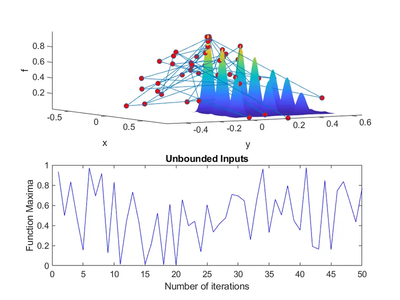
Here the optimal values are exceeding the x and y limits so the global maxima is not clearly achieved.
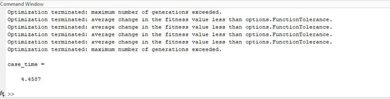
Time taken for the loop to run is =4.4587s
CASE 2 - STATISTICAL BEHAVIOR OF STALAGMITE FUNCTION WITH UPPER AND LOWER BOUND LIMITS.
Here we are going to solve the stalagmite function with upper and lower bound limits. We are doing this to narrow the search for maxima and to have less fluctuations for more accurate result of the maxima.
Program2:
clear all % used to clear the variables in the workspace
close all %used  to close all the figure windows
clc %used to clear the command window

%defining our search space by giving variables within our desired range
x= linspace(0,0.6,150);
y= linspace(0,0.6,150);

cases=50; %this is the number of iterations you want the genetic algorithm to run

%creating a two dimensional mesh
[xx yy]=meshgrid(x,y);

%Evaluating the stalgamite function

for i=1:length(xx)
%it shows the number of times you want the loop to run in this case from 1 to length of the 'xx' array.

for j=1:length(yy)
%it shows the number of times you want the loop to run in this case from 1 to length of the 'yy' array.

input_vector(1)=xx(i,j);
input_vector(2)=yy(i,j);
%here each time the loop runs the value of 'xx' and 'yy' is taken and input into variables respectively.

f(i,j)=stalagmite(input_vector);% here we are calling the stalagmite function with the values of 'xx' and 'yy'
end
end % end of for loop

%statistical behavior

tic % stopwatch timer starts

for i=1:cases %here the loop runs from 1 to till the defined number of cases.
[inputs,fopt(i)]=ga(@stalagmite,2,[],[],[],[],[0;0],[0.6;0.6]);
%here function is called with '@' and 'ga' which is a inbuilt solver in matlab is used to solve the stalagmite function with the inputs we have provided.And the outputs will be saved in 2 arrays ' inputs' and fopt(i).And the boundary conditions of upper and lower bound limits are also added.

xopt(i)=inputs(1);
yopt(i)=inputs(2);
%here the optimal values of inputs are stored in 'xopt' and 'yopt' for every iteration of the loop.

end %end of loop
case_time=toc %time taken by the loop to calculate optimal values is calculated and output is given with the variable'case_time'

%plotting according to the genetic algorithm statistical behavior

subplot(2,1,1)%subplot is used to create more than one graph in the same window with 2 columns and 1 row.
hold on % hold or retain the plot
surfc(x,y,-f)% used to create 3 dimensional subplot.
shading interp % used for the smootheness of the surface.
plot3(xopt,yopt,-fopt,'marker','o','markersize',5,'markerfacecolor','red')% is used to create the optimal 'x' and 'y' and function values in the 3-D plot
xlabel('x')
ylabel('y')
zlabel('f')
%for labling of 'x','y' and 'f'.
subplot(2,1,2)
plot(-fopt,'color','b')%plotting to observe the variation with respectto optimal function value.
title('Bounded Inputs')%title for the graph.
xlabel('Number of iterations')%x axis labling.
ylabel('Function Maxima')%y axis labling.
OUTPUT2:
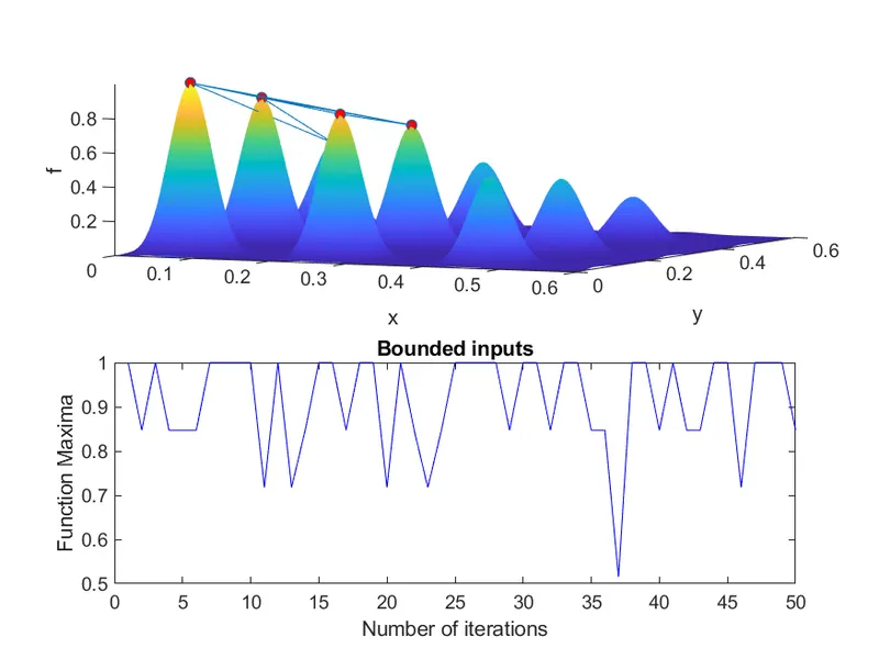
Here the optimal values are shown within the x and y limits with lesser fluctuations but yet global maxima is not clearly shown.
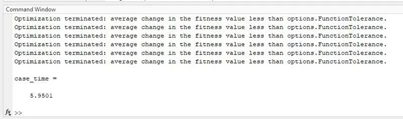
Time taken for the loop to run is =5.9501s
CASE 3 - STATISTICAL BEHAVIOR OF STALAGMITE FUNCTION WITH SPECIFICATION OF POPULATION SIZE AND UPPER AND LOWER BOUND LIMITS.
Here we are going to use the options command as we are going to modify the population size.
PROGRAM3:
clear all % used to clear the variables in the workspace
close all %used  to close all the figure windows
clc %used to clear the command window

%defining our search space by giving variables within our desired range
x= linspace(0,0.6,150);
y= linspace(0,0.6,150);

cases=50; %this is the number of iterations you want the genetic algorithm to run

%creating a two dimensional mesh
[xx yy]=meshgrid(x,y);

%Evaluating the stalgamite function

for i=1:length(xx)
%it shows the number of times you want the loop to run in this case from 1 to length of the 'xx' array.

for j=1:length(yy)
%it shows the number of times you want the loop to run in this case from 1 to length of the 'yy' array.

input_vector(1)=xx(i,j);
input_vector(2)=yy(i,j);
%here each time the loop runs the value of 'xx' and 'yy' is taken and input into variables respectively.

f(i,j)=stalagmite(input_vector);% here we are calling the stalagmite function with the values of 'xx' and 'yy'
end
end % end of for loop

%increasing the population size with the help of options command.
options=optimoptions('ga');%options command with solver name.
options=optimoptions(options,'populationsize',500);

%statistical behavior

tic % stopwatch timer starts

for i=1:cases %here the loop runs from 1 to till the defined number of cases.
[inputs,fopt(i)]=ga(@stalagmite,2,[],[],[],[],[0;0],[0.6;0.6],[],[],options);
%here function is called with '@' and 'ga' which is a inbuilt solver in matlab is used to solve the stalagmite function with the inputs we have provided.And the outputs will be saved in 2 arrays ' inputs' and fopt(i).And the boundary conditions of upper and lower bound limits are also added.

xopt(i)=inputs(1);
yopt(i)=inputs(2);
%here the optimal values of inputs are stored in 'xopt' and 'yopt' for every iteration of the loop.

end %end of loop
case_time=toc %time taken by the loop to calculate optimal values is calculated and output is given with the variable'case_time'

%plotting according to the genetic algorithm statistical behavior

subplot(2,1,1)%subplot is used to create more than one graph in the same window with 2 columns and 1 row.
hold on % hold or retain the plot
surfc(x,y,-f)% used to create 3 dimensional subplot.
shading interp % used for the smootheness of the surface.
plot3(xopt,yopt,-fopt,'marker','o','markersize',5,'markerfacecolor','red')% is used to create the optimal 'x' and 'y' and function values in the 3-D plot
xlabel('x')
ylabel('y')
zlabel('f')
%for labling of 'x','y' and 'f'.
subplot(2,1,2)
plot(-fopt,'color','b')%plotting to observe the variation with respectto optimal function value.
title('statistical behavior with population size')%title for the graph.
xlabel('Number of iterations')%x axis labling.
ylabel('Function Maxima')%y axis labling.
OUTPUT3:
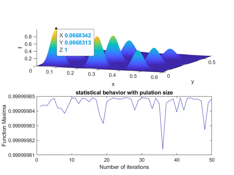
As we can see above the global maxima value is centered at the peak on only one point thus the global maxima is achieved here. And the point of global maxima is x=0.0668342,y=0.0668313,z=1.
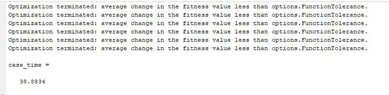
Time taken for the loop to run =38.8834s.
ERRORS:
Error1:
I used the marker as '0' instead of 'o' and corrected it after the error occured.

Error2:
I added an extra bracket wich allowed the error to occcur later i removed the extra bracket.

Error3:
I gave a space inbetween the string later after the error occured i corrected it.

RESULT:
Thus the optimization of stalagmite function is done successfully and its global maxima value is also achieved and shown above with the help of the plot.And the plots for each case is shown above separately.
CONCLUSION:
Thus by increasing the number of iterations and increasing the population size the global maxima of the stalagmite function is achieved with accuracy.