Project 2 - Rankine cycle Simulator
RANKINE CYCLE SIMULATOR USING MATLAB.
AIM:
To create a Rankine cycl simulator using Matlab and calculate the state points based on the user inputs. And also plot the T-S and H-S relation diagram.
CONTENTS:
- EXPLANATION OF RANKINE CYCLE.
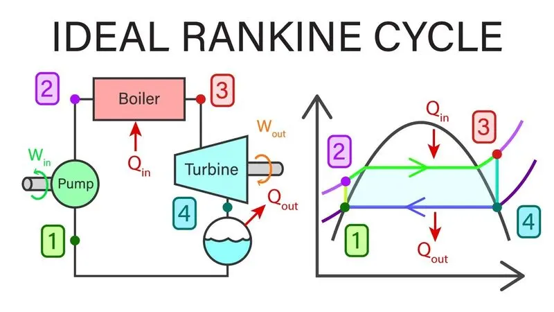
- IDEAL RANKINE CYCLE DIAGRAM.
- TERMINOLOGIES USED.
- PROGRAM.
- STEP-WISE EXPLANATION OF THE CODE.
- RESULT.
- ERRORS.
- CONCLUSION,
- REFERENCES.
EXPLANATION OF RANKINE CYCLE:
The Rankine cycle is an idealized thermodynamic cycle describing the process by which certain heat engines, such as steam turbines or reciprocating steam engines, allow mechanical work to be extracted from a fluid as it moves between a heat source and heat sink.
Heat energy is supplied to the system via a boiler where the working fluid (typically water) is converted to a high pressure gaseous state (steam) in order to turn a turbine. After passing over the turbine the fluid is allowed to condense back into a liquid state as waste heat energy is rejected before being returned to the boiler, completing the cycle. Friction losses throughout the system are often neglected for the purpose of simplifying calculations as such losses are usually much less significant than thermodynamic losses, especially in larger systems.
The Rankine cycle closely describes the process by which steam engines commonly found in thermal power generation plants harness the thermal energy of a fuel or other heat source to generate electricity. Possible heat sources include combustion of fossil fuels such as coal natural gas or oil, renewable fuels like biomass or ethanol, nuclear fission or fusion, and concentrated solar power. Common heat sinks include ambient air above or around a facility and bodies of water such as rivers, ponds, and oceans.The ability of a Rankine engine to harness energy depends on the relative temperature difference between the heat source and heat sink. The greater the differential, the more mechanical power can be efficiently extracted out of heat energy, as per Carnots theoremThe efficiency of the Rankine cycle is limited by the high heat of vaporization of the working fluid. Unless the pressure and temperature reach super critical levels in the boiler the temperature range, that the cycle can operate over, is quite small: Steam turbine entry temperatures are typically around 565 °C and condenser temperatures are around 30 °C.
THE FOUR PROCESS IN A RANKINE CYCLE:
- Process 1–2: The working fluid is pumped from low to high pressure. As the fluid is a liquid at this stage, the pump requires little input energy.
In other words, Process 1-2 is [Isentropic compression].
- Process 2–3: The high-pressure liquid enters a boiler, where it is heated at constant pressure by an external heat source to become a dry saturated vapour. The input energy required can be easily calculated graphically, using an enthalpy-entropy chart or numerically, using team tables.
In other words, Process 2-3 is [Isobaric heat addition/Constant pressure heat addition in boiler].
- Process 3–4: The dry saturated vapour expands through a turbine, generating power. This decreases the temperature and pressure of the vapour, and some condensation may occur. The output in this process can be easily calculated using the chart or tables noted above.
In other words, Process 3-4 is [Isentropic expansion].
- Process 4–1: The wet vapour then enters a condenser, where it is condensed at a constant pressure to become a saturated liquid.
In other words, Process 4-1 is [Isobaric heat rejection/Constant pressure heat rejection in condenser].
TERMINOLOGIES USED:
Work done on pump, per kg of water, WP= h2-h1.
Energy added in steam generator, q1= h3-h2.
Work delivered by turbine,WT = H4 – H3.
Energy rejected in the condenser, q2= h4-h1.
The thermal efficiency of the Rankine cycle is given by,
Efficiency= (q1-q2)/q1=(h3-h2)-(h4-h1)/h3-h2
Efficiency= Net work done.
hL_p-enthalpy of liquid at constant pressure.
hV_p-enthalpy of vapour at constant pressure.
T_ph-temperature as a function of pressure and enthalpy.
h_pT-enthalpy as a function of pressure and temperature..
sL_p-enthalpy of liquid at constant pressure.
sV_p-enthalpy of vapour at constant pressure.
Tsat_p-saturation temperature
PROGRAM:
close all
clear all
clc
%Header
disp(' RANKINE CYCLE STIMULATION' );
disp('1-2 Isentropic expanion in the turine.');
disp('2-3 Constant pressure heat rejection by condenser.');
disp('3-4 Isentropic compression of the pump.');
disp('4-5 Constant pressure heat addition.');
fprintf('\n');

%user inputs
t1=input('Enter the turbine inlet Temperature in degree C: ');
p1=input('Enter the turbine inlet Pressure in Bar: ');
p2=input('Enter the turbine outlet Pressure in Bar: ');
fprintf('\n');

%gamma value which constant value
gamma=1.4

%State 1 ( Turbine inlet)

h1=XSteam('h_pT',p1,t1);
s1=XSteam('s_pT',p1,t1);
hl1_sat=XSteam('hL_p',p1);
hg1_sat=XSteam('hV_p',p1);
sl1_sat=XSteam('sL_p',p1);
sg1_sat=XSteam('sV_p',p1);
T_sat1=XSteam('Tsat_p',p1);
%process 1-2 Isentropic Expansion in the Turbine s1=s2
%For isentropic process (pv)^gamma=constant(p1/p2)=(v2/v1)^gamma

%state 2 (condenser inlet)
s2=s1;
sl2_sat=XSteam('sL_p',p2);
sg2_sat=XSteam('sV_p',p2);
%drynes fraction 'X' calculation
x=(s2-sl2_sat)/(sg2_sat-sl2_sat);
hl2_sat=XSteam('hL_P',p2);
hg2_sat=XSteam('hV_P',p2);
T_sat2=XSteam('Tsat_p',p2);
h2=hl2_sat+x*(hg2_sat-hl2_sat);
t2=XSteam('T_ph',p2,h2);

%state 3(pump inlet)
p3=p2;
t3=t2;
s3=sl2_sat;
h3=hl2_sat;

%state 4  (boiler inlet)
s4=s3;
p4=p1;
t4=XSteam('T_ps',p4,s4);
h4=XSteam('h_ps',p4,s4);

%plots
%T-S plot for rankine cycle
figure(1)
hold on
t=linspace(0,373.15,500);
for i=1:length(t)
    plot(XSteam('sL_T',t(i)),t(i),'g.');
    plot(XSteam('sV_T',t(i)),t(i),'r.');
end

plot([s1,s2],[t1,t2],'linewidth',2);
text(s1,t1,'1','FontSize',20);
if x>1;
    t3=T_sat2
plot([s2 sg2_sat s3 s4],[t2 T_sat2 t3 t4],'linewidth',2,'color','b');
text(s1,t2,'2','FontSize',20);
text(s3,t3,'3','FontSize',20);
else
plot([s2 s3 s4],[t2 t3 t4],'linewidth',2,'color','b');
text(s1,t2,'2','FontSize',20);
text(s3,t3,'3','FontSize',20);
end

n=linspace(t1,t2,500);
for i=1:length(n)
    plot(XSteam('s_pT',p1,n(i)),n(i),'.','linewidth',2,'color','b');
end

plot([sl1_sat sg1_sat],[T_sat1 T_sat1],'linewidth',2,'color','b');
text(sl1_sat,T_sat1,'4','FontSize',20);
    xlabel('Entropy(KJ/KgK)')
    ylabel('Temprature(K)')
    legend('Liquid saturation curve','vapour saturation curve');
    title('T-S Relation')


%H-S Relation
figure(2)
hold on
for i=1:length(t)
plot(XSteam('sL_T',t(i)),XSteam('hL_T',t(i)),'g.');
plot(XSteam('sV_T',t(i)),XSteam('hV_T',t(i)),'r.');
plot([s1 s2 s3 s4 s1],[h1 h2 h3 h4 h1],'linewidth',2,'color','b');
end

text(s1,h1,'1','Fontsize',20)
text(s2,h2,'2','Fontsize',20)
text(s3,h3,'3','Fontsize',20)
text(s4,h4,'4','Fontsize',20)
xlabel('Entropy(KJ/KgK)')
ylabel('Temprature(K)')
legend('Liquid saturation curve','vapour saturation curve');
title('H-S Relation')

%work calculation
wt=h1-h2;
wp=h4-h3;
wnet=wt-wp;
ntherm=wnet/(h1-h4)*100;
back_work=wp/wt;
ssc=3600/wnet

%command diplay

disp(' Result ')
fprintf('\n')
disp('AT STATE POINT 1')
fprintf('\n')
P1=sprintf('P1 is : %.5f Bar',p1);
disp(P1);
T1=sprintf('T1 is : %.5f degree C',t1);
disp(T1);
H1=sprintf('H1 is : %.5f KJ/Kg',h1);
disp(H1);
S1=sprintf('S1 is : %.5f KJ/KgK',s1);
disp(S1);
fprintf('\n')

disp('AT STATE POINT 2')
fprintf('\n')
P2=sprintf('P2 is : %.5f Bar',p2);
disp(P2);
T2=sprintf('T2 is : %.5f degree C',t2);
disp(T2);
H2=sprintf('H2 is : %.5f KJ/Kg',h2);
disp(H2);
S2=sprintf('S2 is : %.5f KJ/KgK',s2);
disp(S2);
fprintf('\n')

disp('AT STATE POINT 3')
fprintf('\n');
P3=sprintf('P3 is : %.5f Bar',p3);
disp(P3);
T3=sprintf('T3 is : %.5f degree C',t3);
disp(T3);
H3=sprintf('H3 is : %.5f KJ/Kg',h3);
disp(H3);
S3=sprintf('S3 is : %.5f KJ/KgK',s3);
disp(S3);
fprintf('\n')

disp('AT STATE POINT 4')
fprintf('\n')
P4=sprintf('P4 is : %.5f Bar',p4);
disp(P4);
T4=sprintf('T4 is : %.5f degree C',t4);
disp(T4);
H4=sprintf('H4 is : %.5f KJ/Kg',h4);
disp(H4);
S4=sprintf('S4 is : %.5f KJ/KgK',s4);
disp(S4);
fprintf('\n');

wt=sprintf('wt is : %5f KJ/Kg',wt);
disp(wt);
wp=sprintf('wp is : %5f KJ/Kg',wp);
disp(wp);
wnet=sprintf('wnet is : %5f KJ/Kg',wnet);
disp(wnet);
ntherm=sprintf('ntherm is : %5f %%',ntherm);
disp(ntherm);
ssc=sprintf('ssc is : %5f Kg/KWh',ssc);
disp(ssc);
STEP WISE EXPLANTION OF THE CODE:
close all
clear all
clc
close all is used to close all the figure windows, clear all is used to clear all the workspace and clc is used to clear the command window.
%Header
disp(' RANKINE CYCLE STIMULATION' );
disp('1-2 Isentropic expanion in the turine.');
disp('2-3 Constant pressure heat rejection by condenser.');
disp('3-4 Isentropic compression of the pump.');
disp('4-1 Constant pressure heat addition.');
Here the header information is displayed using the 'disp' function which is an inbuilt function in matlab. Each cycle or stage of rankine cycle is displayed.
%user inputs
t1=input('Enter the turbine inlet Temperature in degree C: ');
p1=input('Enter the turbine inlet Pressure in Bar: ');
p2=input('Enter the turbine outlet Pressure in Bar: ');
fprintf('\n');
Here the values of 't1,p1 and p2' are left for the user to input . so they are basically user inputs . With the help of 'input' function this operation of user input is carried on. 'frpintf('\n')' forms a new line.
%gamma value which constant value
gamma=1.4
gamma value 1.4 which is a constant value is input into the variable gamma.
%State 1 ( Turbine inlet)

h1=XSteam('h_pT',p1,t1);
s1=XSteam('s_pT',p1,t1);
hl1_sat=XSteam('hL_p',p1);
hg1_sat=XSteam('hV_p',p1);
sl1_sat=XSteam('sL_p',p1);
sg1_sat=XSteam('sV_p',p1);
T_sat1=XSteam('Tsat_p',p1);
%process 1-2 Isentropic Expansion in the Turbine s1=s2
%For isentropic process (pv)^gamma=constant(p1/p2)=(v2/v1)^gamma

%state 2 (condenser inlet)
s2=s1;
sl2_sat=XSteam('sL_p',p2);
sg2_sat=XSteam('sV_p',p2);
%drynes fraction 'X' calculation
x=(s2-sl2_sat)/(sg2_sat-sl2_sat);
hl2_sat=XSteam('hL_P',p2);
hg2_sat=XSteam('hV_P',p2);
T_sat2=XSteam('Tsat_p',p2);
h2=hl2_sat+x*(hg2_sat-hl2_sat);
t2=XSteam('T_ph',p2,h2);

%state 3(pump inlet)
p3=p2;
t3=t2;
s3=sl2_sat;
h3=hl2_sat;

%state 4  (boiler inlet)
s4=s3;
p4=p1;
t4=XSteam('T_ps',p4,s4);
h4=XSteam('h_ps',p4,s4);
Here state point propertie are calculated by steam table function 'XSteam', The XSteam data library is stored in the same directory where the program is coded and then using 'XSteam' function the values are dervied for calculation.
%plots
%T-S plot for rankine cycle
figure(1)
hold on
t=linspace(0,373.15,500);
for i=1:length(t)
    plot(XSteam('sL_T',t(i)),t(i),'g.');
    plot(XSteam('sV_T',t(i)),t(i),'r.');
end

plot([s1,s2],[t1,t2],'linewidth',2);
text(s1,t1,'1','FontSize',20);
if x>1;
    t3=T_sat2
plot([s2 sg2_sat s3 s4],[t2 T_sat2 t3 t4],'linewidth',2,'color','b');
text(s1,t2,'2','FontSize',20);
text(s3,t3,'3','FontSize',20);
else
plot([s2 s3 s4],[t2 t3 t4],'linewidth',2,'color','b');
text(s1,t2,'2','FontSize',20);
text(s3,t3,'3','FontSize',20);
end

n=linspace(t1,t2,500);
for i=1:length(n)
    plot(XSteam('s_pT',p1,n(i)),n(i),'.','linewidth',2,'color','b');
end

plot([sl1_sat sg1_sat],[T_sat1 T_sat1],'linewidth',2,'color','b');
text(sl1_sat,T_sat1,'4','FontSize',20);
    xlabel('Entropy(KJ/KgK)')
    ylabel('Temprature(K)')
    legend('Liquid saturation curve','vapour saturation curve');
    title('T-S Relation')


%H-S Relation
figure(2)
hold on
for i=1:length(t)
plot(XSteam('sL_T',t(i)),XSteam('hL_T',t(i)),'g.');
plot(XSteam('sV_T',t(i)),XSteam('hV_T',t(i)),'r.');
plot([s1 s2 s3 s4 s1],[h1 h2 h3 h4 h1],'linewidth',2,'color','b');
end

text(s1,h1,'1','Fontsize',20)
text(s2,h2,'2','Fontsize',20)
text(s3,h3,'3','Fontsize',20)
text(s4,h4,'4','Fontsize',20)
xlabel('Entropy(KJ/KgK)')
ylabel('Temprature(K)')
legend('Liquid saturation curve','vapour saturation curve');
title('H-S Relation')
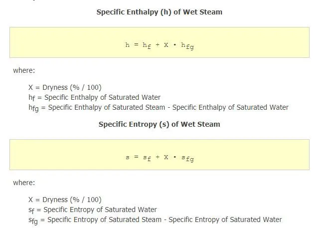
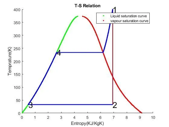
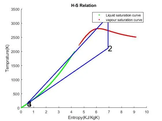
Here T-S and H-S relation are plotted using 'plot' command and all the process cycle are numbered using 'text' command and their respective x-asis , y-axis and title are given using ' text,xlabel and ylabel' commands.
%work calculation
wt=h1-h2;
wp=h4-h3;
wnet=wt-wp;
ntherm=wnet/(h1-h4)*100;
back_work=wp/wt;
ssc=3600/wnet
Here the work done by the turbine and the pump are calculated , and using those two inputs the net work done and back work rate is also calculated.
%command diplay

disp(' Result ')
fprintf('\n')
disp('AT STATE POINT 1')
fprintf('\n')
P1=sprintf('P1 is : %.5f Bar',p1);
disp(P1);
T1=sprintf('T1 is : %.5f degree C',t1);
disp(T1);
H1=sprintf('H1 is : %.5f KJ/Kg',h1);
disp(H1);
S1=sprintf('S1 is : %.5f KJ/KgK',s1);
disp(S1);
fprintf('\n')

disp('AT STATE POINT 2')
fprintf('\n')
P2=sprintf('P2 is : %.5f Bar',p2);
disp(P2);
T2=sprintf('T2 is : %.5f degree C',t2);
disp(T2);
H2=sprintf('H2 is : %.5f KJ/Kg',h2);
disp(H2);
S2=sprintf('S2 is : %.5f KJ/KgK',s2);
disp(S2);
fprintf('\n')

disp('AT STATE POINT 3')
fprintf('\n');
P3=sprintf('P3 is : %.5f Bar',p3);
disp(P3);
T3=sprintf('T3 is : %.5f degree C',t3);
disp(T3);
H3=sprintf('H3 is : %.5f KJ/Kg',h3);
disp(H3);
S3=sprintf('S3 is : %.5f KJ/KgK',s3);
disp(S3);
fprintf('\n')

disp('AT STATE POINT 4')
fprintf('\n')
P4=sprintf('P4 is : %.5f Bar',p4);
disp(P4);
T4=sprintf('T4 is : %.5f degree C',t4);
disp(T4);
H4=sprintf('H4 is : %.5f KJ/Kg',h4);
disp(H4);
S4=sprintf('S4 is : %.5f KJ/KgK',s4);
disp(S4);
fprintf('\n');

wt=sprintf('wt is : %5f KJ/Kg',wt);
disp(wt);
wp=sprintf('wp is : %5f KJ/Kg',wp);
disp(wp);
wnet=sprintf('wnet is : %5f KJ/Kg',wnet);
disp(wnet);
ntherm=sprintf('ntherm is : %5f %%',ntherm);
disp(ntherm);
ssc=sprintf('ssc is : %5f Kg/KWh',ssc);
disp(ssc);
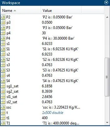
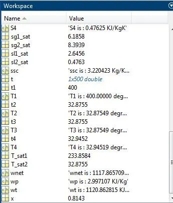
Here all the state point values and work outputs values are displayed in the command window using the 'disp' command which displays all the values.
RESULTS:
PLOT :
COMMAND WINDOW:
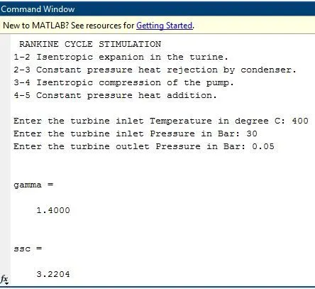
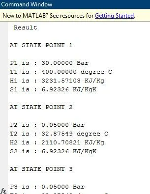
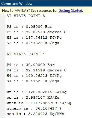
WORKSPACE:
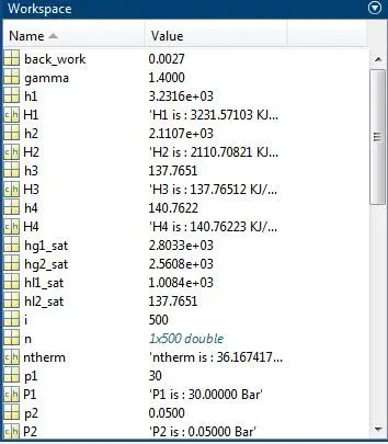
ERRORS:
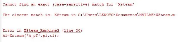
i intially did a case sensitive error , and then once the error occured i recitified it.
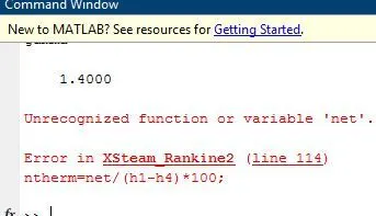
i gave a wrong variable then later after the error occured i corrected it into correct variable.
CONCLUSION:
Hence the by using the above matlab code the rankine cycle can be simulated with the help of use inputs and results shown are accurate.
REFERENCE:
https://www.sciencedirect.com/topics/engineering/back-work-ratio