Week 4.1 - Genetic Algorithm
Aim:
To write a code in MATLAB to optimize the stalagmite function and find the global maxima of the function.
Objectives:
- To explain the genetic algorithm and its syntax.
- Write a code to optimize the stalagmite function.
- Find the global maxima of the function.
Theory:
GENETIC ALGORITHM:
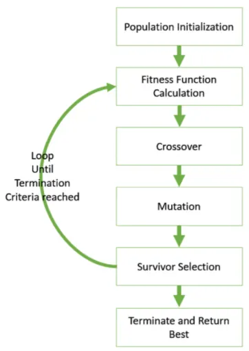
The genetic algorithm is inspired by the process that drives biological evolution. The process of evolution starts with the selection of the fittest individuals from a population. Then they produce offspring that inherit the parents' characteristics and will be added to the next generation. If parents have better fitness, their offspring will be better than parents and have a better chance of surviving. This process keeps on iterating and in the end, a generation with the fittest individuals will be found. And this is th main working principle for the algorithm because, at each step, the genetic algorithm selects randomly from the current population to be parents and uses them to produce the children for the next generation. Over successive generations, the population evolves toward an optimal solution. The genetic algorithm can be applied to solve a variety of optimization problems that are not well suited for standard optimization algorithms, including problems in which the objective function is discontinuously nondifferentiable, stochastic, or highly nonlinear.
The genetic algorithm uses three main types of rules at each step to create the next generation from the current population:
- Selection rules select the individuals, called parents, that contribute to the population at the next generation.
- Crossover rules combine two parents to form children for the next generation.
- Mutation rules apply random changes to individual parents to form children.
Genetic Algorithm Syntax:
For Random Inputs:
x = ga(fun,nvars) finds a local unconstrained minimum, x, to the objective function, fun. nvars is the dimension (number of design
variables) of fun.
For Bounded Inputs:
x = ga(fun,nvars,A,b,Aeq,beq,lb,ub) defines a set of lower and upper bounds on the design variables, x, so that a solution is found
in the range lb ≤ x ≤ ub. (Set Aeq= [] and beq= [] if no linear equalities exist.)
For Population size:
x = ga(fun,nvars,A,b,[],[],lb,ub,nonlcon,IntCon,options) requires that the variables listed in IntCon take integer values.
Where,
Fun - function,
Nvars – Number of Variables
A – Linear inequality constraints
B – Linear inequality constraints
Aeq - linear equality constraints
beq – linear equality constraints
lb – lower Bounds
ub – Upper Bounds
nonlcon – Non- Linear Constraints
IntCon – Integer Constraints
Equations Used:
The Function is for the Genetic Algorithm of the global minima, but to attain the maxima value, the ‘-’ is placed before the equation.
f(x, y) = f1 . x × f2 . x × f1 . y × f2 . y
Where,
f1 . x = [sin(5.1πx + 0.5)]6
f1 . y = [sin(5.1πy + 0.5)]6
f2 . x = exp[ − 4 ln(2) × ](x − 0.0667)20.64
f2 . y = exp[ − 4 ln(2) × ](y − 0.0667)20.64
The Global maxima is as follows
f(x, y) = − (f1 . x × f2 . x × f1 . y × f2 . y)
Coding:
Stalagmite Function:
% Stalagmite function
function[f] = stalagmite(input_vector)
x = input_vector(1);
y = input_vector(2);

f1 = (sin(5.1*pi*x+0.5)).^6;
f2 = exp(-4*log(2)*((x-0.0667).^2)./0.64);
f3 = (sin(5.1*pi*y+0.5)).^6;
f4 = exp(-4*log(2)*((y-0.0667).^2)./0.64);

f = -(f1*f2*f3*f4);
end
Unbounded Inputs:
% Unbounded
clear all
close all
clc

x = linspace(0,0.6,120);
y = linspace(0,0.6,120);

[xx yy]=meshgrid(x,y);
num_cases = 50

%study1- Statistical Behaviour (unbounded)
for i = 1:length(xx)
 for j = 1:length(yy)

 input_vector(1) = xx(i,j);
 input_vector(2) = yy(i,j);

 f(i,j) = stalagmite(input_vector);

 end
end

tic
for i=1:num_cases
    [inputs,fopt(i)] = ga(@stalagmite,2);
    xopt(i) = inputs(1);
    yopt(i) = inputs(2);

end
study1_time = toc

figure(1)
subplot(2,1,1)
hold on
surfc(x,y,f)
shading interp
plot3(xopt,yopt,fopt,'marker','o','markersize',5,'markerfacecolor','r')
title('Unbounded Inputs')
subplot(2,1,2)
plot(fopt)
xlabel('Iterations')
ylabel('Function minimum')
Study time: 4.5230
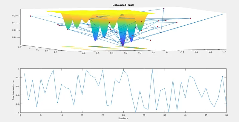
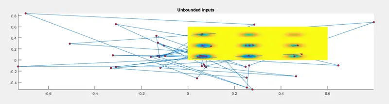
Graph:
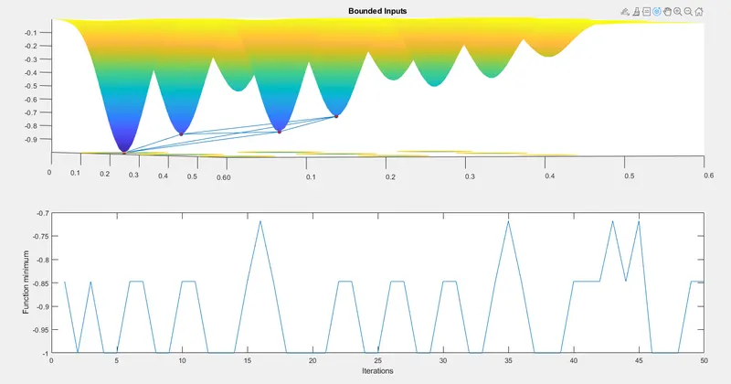
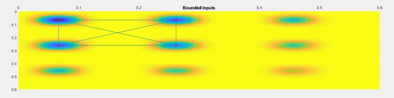
Bounded Inputs with upper and lower bound:
% Bounded
clear all
close all
clc

x = linspace(0,0.6,120);
y = linspace(0,0.6,120);

[xx yy]=meshgrid(x,y);
num_cases = 50

%study2- Statistical Behaviour with upper aqnd lower bounds(Bounded)
for i = 1:length(xx)
 for j = 1:length(yy)

 input_vector(1) = xx(i,j);
 input_vector(2) = yy(i,j);

 f(i,j) = stalagmite(input_vector);

 end
end

tic
for i=1:num_cases
    [inputs,fopt(i)] = ga(@stalagmite,2,[],[],[],[],[0,0],[1,1]);
    xopt(i) = inputs(1);
    yopt(i) = inputs(2);

end
study2_time = toc

figure(1)
subplot(2,1,1)
hold on
surfc(x,y,f)
shading interp
plot3(xopt,yopt,fopt,'marker','o','markersize',5,'markerfacecolor','r')
title('Bounded Inputs')
subplot(2,1,2)
plot(fopt)
xlabel('Iterations')
ylabel('Function minimum')
Study time: 5.9746
Graph:
Statistical Behaviour with an increase in population:
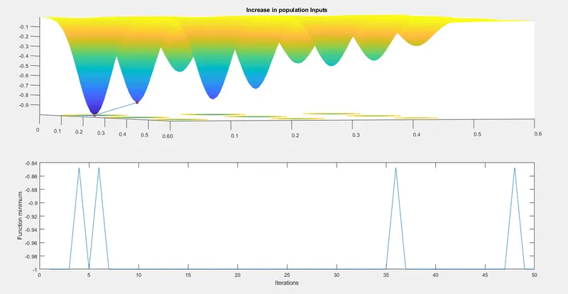
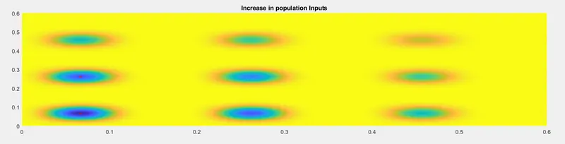
% Increase in population
clear all
close all
clc

x = linspace(0,0.6,120);
y = linspace(0,0.6,120);

[xx yy]=meshgrid(x,y);
num_cases = 50

%study3- Statistical Behaviour with increase in population (Bounded)
for i = 1:length(xx)
 for j = 1:length(yy)

 input_vector(1) = xx(i,j);
 input_vector(2) = yy(i,j);

 f(i,j) = stalagmite(input_vector);

 end
end
options = optimoptions('ga');
options = optimoptions(options,'populationsize',150);

tic
for i=1:num_cases
    [inputs,fopt(i)] = ga(@stalagmite,2,[],[],[],[],[0,0],[1,1],[],[],options);
    xopt(i) = inputs(1);
    yopt(i) = inputs(2);

end
study3_time = toc

figure(1)
subplot(2,1,1)
hold on
surfc(x,y,f)
shading interp
plot3(xopt,yopt,fopt,'marker','o','markersize',5,'markerfacecolor','r')
title('Increase in population Inputs')
subplot(2,1,2)
plot(fopt)
xlabel('Iterations')
ylabel('Function minimum')
Study time: 11.8362
Graph:
Main code:
clear all
close all
clc

x = linspace(0,0.6,120);
y = linspace(0,0.6,120);

[xx yy]=meshgrid(x,y);
num_cases = 50

%study1- Statistical Behaviour (unbounded)
for i = 1:length(xx)
 for j = 1:length(yy)

 input_vector(1) = xx(i,j);
 input_vector(2) = yy(i,j);

 f(i,j) = stalagmite(input_vector);

 end
end

tic
for i=1:num_cases
    [inputs,fopt(i)] = ga(@stalagmite,2);
    xopt(i) = inputs(1);
    yopt(i) = inputs(2);

end
study1_time = toc

figure(1)
subplot(2,1,1)
hold on
surfc(x,y,f)
shading interp
plot3(xopt,yopt,fopt,'marker','o','markersize',5,'markerfacecolor','r')
title('Unbounded Inputs')
subplot(2,1,2)
plot(fopt)
xlabel('Iterations')
ylabel('Function minimum')

%study2- Statistical Behaviour with upper aqnd lower bounds(Bounded)
for i = 1:length(xx)
 for j = 1:length(yy)

 input_vector(1) = xx(i,j);
 input_vector(2) = yy(i,j);

 f(i,j) = stalagmite(input_vector);

 end
end

tic
for i=1:num_cases
    [inputs,fopt(i)] = ga(@stalagmite,2,[],[],[],[],[0,0],[1,1]);
    xopt(i) = inputs(1);
    yopt(i) = inputs(2);

end
study2_time = toc

figure(2)
subplot(2,1,1)
hold on
surfc(x,y,f)
shading interp
plot3(xopt,yopt,fopt,'marker','o','markersize',5,'markerfacecolor','r')
title('Bounded Inputs')
subplot(2,1,2)
plot(fopt)
xlabel('Iterations')
ylabel('Function minimum')

%study3- Statistical Behaviour with increase in population (Bounded)
for i = 1:length(xx)
 for j = 1:length(yy)

 input_vector(1) = xx(i,j);
 input_vector(2) = yy(i,j);

 f(i,j) = stalagmite(input_vector);

 end
end
options = optimoptions('ga');
options = optimoptions(options,'populationsize',150);

tic
for i=1:num_cases
    [inputs,fopt(i)] = ga(@stalagmite,2,[],[],[],[],[0,0],[1,1],[],[],options);
    xopt(i) = inputs(1);
    yopt(i) = inputs(2);

end
study3_time = toc

figure(3)
subplot(2,1,1)
hold on
surfc(x,y,f)
shading interp
plot3(xopt,yopt,fopt,'marker','o','markersize',5,'markerfacecolor','r')
title('Increase in population Inputs')
subplot(2,1,2)
plot(fopt)
xlabel('Iterations')
ylabel('Function minimum')

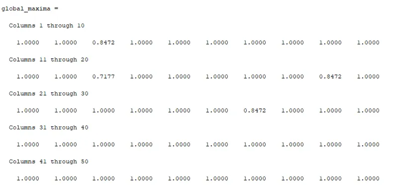
global_maxima = -fopt
Results:
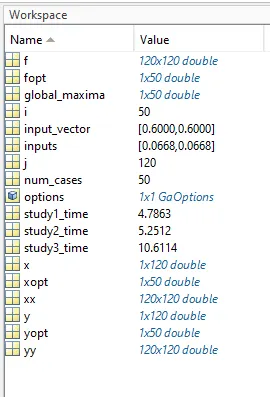
Workspace: