Week 4.1 - Genetic Algorithm
AIM: Write a code in MATLAB to optimise the stalagmite function and find the global maxima of the function.
OBJECTIVES:
1.To expalin the concept of genetic algorithm and also explain the syntax for ga in MATLAB.
2.To Plot graphs for all 3 studies and for F maximum vs no. of iterations.
THEORY:
Concept of genetic Algorithm:
- A genetic algorithm (GA) is a method for solving both constrained and unconstrained optimization problems based on a natural selection process that mimics biological evolution. The algorithm repeatedly modifies a population of individual solutions. At each step, the genetic algorithm randomly selects individuals from the current population and uses them as parents to produce the children for the next generation. Over successive generations, the population "evolves" toward an optimal solution.
- You can apply the genetic algorithm to solve problems that are not well suited for standard optimization algorithms, including problems in which the objective function is discontinuous, nondifferentiable, stochastic, or highly nonlinear.
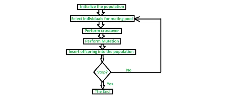
- There are five phases involved in genetic algorithm, which are given as below.
- 1. Initial Population 2.Fitness Function 3.Selection 4.Crossover 5.Mutation
- 1.Initial Population :- Code generates random number of population and according to the fitness of the members from the population according to which it forms new population based on number of iterations performed.
- 2.Fitness Function :- It is the function which we have to optimize based on number of iterations performed.
- 3.Selection :-In this phase, fittest individuals are selected and ga allowed them to pass the genes to the next generation. Purpose behind executing this step is to find out the region where best solution exists.
- 4.Crossover :- Generation of offspring happenes in two ways which are crossover and mutation.During crossover a random point is selected while mating pair of parents to generate offspring.
- 5.Mutation :- In this stage , newly formed offspring is subjected to formed new offspings to maintain diversity among the population.
BODY OF THE CONTENT:
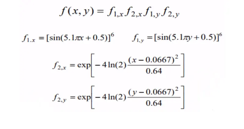
Stalagmite function is given as
Stalagmite Function code :
- Above expressions are used in the stalagmite function to plot a graph in the main functions.
- Inside the code negative sign is included for f variable which will give maximum value of the function.
function [f] = stalagmite(input_vector)

x=input_vector(1);
y=input_vector(2);

f1_x=(sin(5.1*pi*x + 0.5)).^6;
f1_y=(sin(5.1*pi*y + 0.5)).^6;

v1=((x-0.0667).^2)/(0.64)
f2_x=exp(-4.*log(2)*v1);

v2=((y-0.0667).^2)/(0.64)
f2_y=exp(-4.*log(2)*v2);

f = -(f1_x.*f2_x.*f1_y.*f2_y);
end
Main code
- In the below code array of x and y is defined containing 150 values each starting from 0 to 0.6.
- Number of iterations are defined as 50 , that means 50 times genetic algorithm will execute.
- Using meshgrid command 2x2 array is generated for x and y.
- Using stalagmite function values of fitness function at each point of the mesh grid formed.
- Surfc command will provide the surface contour of the function.
close all
clear all
clc

%inputs
x=linspace(0,0.6,150)
y=linspace(0,0.6,150)
num_cases=50;
[X Y]=meshgrid(x,y);

%Creating a surface plot of stalagmite function

for i=1:length(X)
    for j=1:length(Y)
        input_vector(1)=X(i,j);
        input_vector(2)=Y(i,j);
        f(i,j)=stalagmite(input_vector);
    end
end
surfc(X,Y,-f)
shading interp
(i) Study 1 - Statistical study without boundation
- In this study ga will select any values for x and y .
- Using tic-toc command time taken for solving the code can be found out.
- Time required to solve the study is stored inside the study1_time variable.
- subplot command is used when more than 2 plots are required to plot inside the figure.
- subplot(2,1,1) that is upper plot shows the global maxima and local minima contour and their x and y values.
- Using plot3 command , 3d plot of optimum values of function are shown with the help of circles which are networked together.
- subplot(2,1,2) plots optimum values of function with respect to number of iterations.
tic
for i=1:num_cases
    [inputs , fopt(i)]=ga(@stalagmite,2);
    xopt(i)=inputs(1);
    yopt(i)=inputs(2);
end
study1_time=toc

figure(1)
subplot(2,1,1)
surfc(X,Y,-f)
hold on
shading interp
plot3(xopt , yopt,-fopt,'marker','o','markersize',5,'markerfacecolor','r');
xlabel('x value')
ylabel('y value')
grid on
subplot(2,1,2)
plot(-fopt);
xlabel('iterations')
ylabel('function maximum value')
Results:
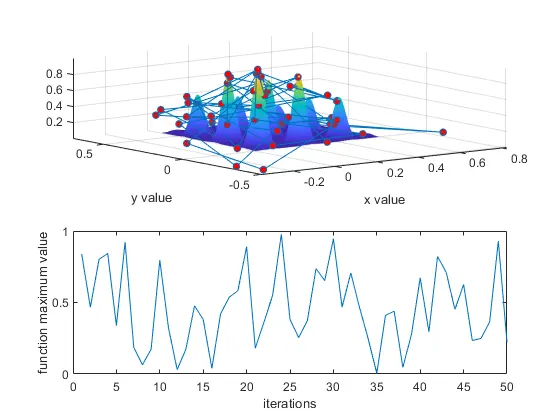
- Above graphs shows optimum value of function is wavering a lot which makes results vague.
Study 2 - Statistical study with Boundation
- This study will run the GA Code for x varies from 0 to 1 and same for y.
- ga(@stalagmite,2,[],[],[],[],[0;0],[1;1]) , In this syntax function name is stalagmite, number of variables are 2, as we don't have any linear constraints hence we have kept next four values as blank([]) and x and y boundries is given in the next two brackets.
- Purpose of giving boundries is to reduced the search space.
- Using tic-toc command time taken for solving the code can be found out.
- Time required to solve the study is stored inside the study2_time variable.
- subplot command is used when more than 2 plots are required to plot inside the figure.
- subplot(2,1,1) that is upper plot shows the global maxima and local minima contour and their x and y values.
- Using plot3 command , 3d plot of optimum values of function are shown with the help of circles which are networked together.
- subplot(2,1,2) plots optimum values of function with respect to number of iterations.
tic
for j=1:num_cases
    [inputs , fopt(j)]=ga(@stalagmite,2,[],[],[],[],[0;0],[1;1]);
    xopt(j)=inputs(1);
    yopt(j)=inputs(2);
end
study2_time=toc

figure(2)
subplot(2,1,1)
surfc(X,Y,-f)
hold on
shading interp
plot3(xopt , yopt,-fopt,'marker','o','markersize',5,'markerfacecolor','r');
xlabel('x value')
ylabel('y value')
grid on
subplot(2,1,2)
plot(-fopt);
xlabel('iterations')
ylabel('function maximum value')
Results
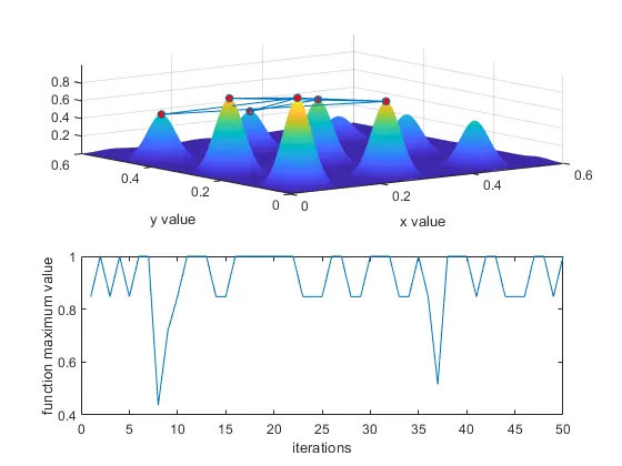
- After providing the boundry value variation in the results is reduced as compared with unbounded study.
Study 3 - Statistical study with increase in size of Population
- This study is more effective as compared with previous two as addition with lower and upper bound we are also defining the population size.
- options = optimoptions('ga','populationsize',300) , This function will pass instruction to ga to select only 300 members for evaluation.
- This type of study is beneficial for processing large data . Only drawback is that time taken will increased.
- Using tic-toc command time taken for solving the code can be found out.
- Time required to solve the study is stored inside the study3_time variable.
- subplot command is used when more than 2 plots are required to plot inside the figure.
- subplot(2,1,1) that is upper plot shows the global maxima and local minima contour and their x and y values.
- Using plot3 command , 3d plot of optimum values of function are shown with the help of circles which are networked together.
- subplot(2,1,2) plots optimum values of function with respect to number of iterations.
options = optimoptions('ga','populationsize',300)
tic
for k=1:num_cases
    [inputs , fopt(k)]=ga(@stalagmite,2,[],[],[],[],[0;0],[1;1],[],[],options);
    xopt(k)=inputs(1);
    yopt(k)=inputs(2);
end
study3_time=toc

figure(3)
subplot(2,1,1)
surfc(X,Y,-f)
hold on
shading interp
plot3(xopt , yopt,-fopt,'marker','o','markersize',5,'markerfacecolor','r');
xlabel('x value')
ylabel('y value')
grid on
subplot(2,1,2)
plot(-fopt);
xlabel('iterations')
ylabel('function maximum value')
Results
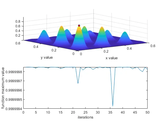
- Among all the three studies , this study shows clear results and variation is also minimal.
Entire Program at once
close all
clear all
clc

%inputs
x=linspace(0,0.6,150)
y=linspace(0,0.6,150)
num_cases=50;
[X Y]=meshgrid(x,y);

%Creating a surface plot of stalagmite function

for i=1:length(X)
    for j=1:length(Y)
        input_vector(1)=X(i,j);
        input_vector(2)=Y(i,j);
        f(i,j)=stalagmite(input_vector);
    end
end
surf(X,Y,-f)
shading interp

%Study 1 - Statistical Study Unbounded
tic
for i=1:num_cases
    [inputs , fopt(i)]=ga(@stalagmite,2);
    xopt(i)=inputs(1);
    yopt(i)=inputs(2);
end
study1_time=toc

figure(1)
subplot(2,1,1)
surfc(X,Y,-f)
hold on
shading interp
plot3(xopt , yopt,-fopt,'marker','o','markersize',5,'markerfacecolor','r');
xlabel('x value')
ylabel('y value')
grid on
subplot(2,1,2)
plot(-fopt);
xlabel('iterations')
ylabel('function maximum value')

%Study 2 - Statistical Study with boundation

tic
for j=1:num_cases
    [inputs , fopt(j)]=ga(@stalagmite,2,[],[],[],[],[0;0],[1;1]);
    xopt(j)=inputs(1);
    yopt(j)=inputs(2);
end
study2_time=toc

figure(2)
subplot(2,1,1)
surfc(X,Y,-f)
hold on
shading interp
plot3(xopt , yopt,-fopt,'marker','o','markersize',5,'markerfacecolor','r');
xlabel('x value')
ylabel('y value')
grid on
subplot(2,1,2)
plot(-fopt);
xlabel('iterations')
ylabel('function maximum value')


%Study 3 - Statistical Study with increase in the size of the population

options = optimoptions('ga','populationsize',300)
tic
for k=1:num_cases
    [inputs , fopt(k)]=ga(@stalagmite,2,[],[],[],[],[0;0],[1;1],[],[],options);
    xopt(k)=inputs(1);
    yopt(k)=inputs(2);
end
study3_time=toc

figure(3)
subplot(2,1,1)
surfc(X,Y,-f)
hold on
shading interp
plot3(xopt , yopt,-fopt,'marker','o','markersize',5,'markerfacecolor','r');
xlabel('x value')
ylabel('y value')
grid on
subplot(2,1,2)
plot(-fopt);
xlabel('iterations')
ylabel('function maximum value')
REFERENCES:
https://skill-lync.com/student-projects/week-4-genetic-algorithm-33
https://in.mathworks.com/discovery/genetic-algorithm.html