Week 3 - Solving second order ODEs

AIM : To solve the Below ODE and animate the motion of pendulum according to the ODE solution

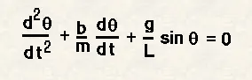
Objectives : 1. To write a program in Matlab to solve above ODE equation.

2. To create an animation of the motion of pendulum.

BODY OF THE CONTENT :

(i)Program to solve above ODE Equation and animate the motion of the pendulum

code

clear all %This command is used to clear the workspace
close all %This command is used to close all the figures
clc

b=0.05; %Damping coefficient
g=9.81; %Gravity in m/s^2
l=1;    %Length of the pendulum in meters
m=1;    %Mass of the pendulum in kg
p1x=0;  %X coordinate of the fixed point
p1y=0;  %Y coordinate of the fixed point

%initial condition
theta_0=[0;3]; %Initial angular displacement is 0 rad and Initial angular velocity is 3 rad/s


%time points
t_span=linspace(0,20,800); %Motion starts from t=0 seconds to t=20 seconds 



%solve ODE
% Below command gives solution of the ODE equation(Displacement and Velocity) with respect to time t.
% Results contain array of two columns which are displacement and velocity.
%ode function(ode_func) is attached at the end of the code named as ode_func
%below funtion ode45 is dependent on two variables t and theta
[t results] = ode45(@(t,theta) ode_func(t,theta,b,g,l,m),t_span , theta_0);



plot(p1x,p1y,'*','color','r')
displacement=[results(:,1)] %Array of displacement is extracted from results and stored in the displacement variable
ct=1 %Defining count as 1


for i=1:length(displacement) %Defining for loop starts from i=1 till last value in the displacement array
p2x=-l*sin(displacement(i)) %Position of Pendulum with respect to X axis
p2y=-l*cos(displacement(i)) %Position of Pendulum with respect to Y axis
plot([p1x p2x] , [p1y p2y] , 'linewidth' , 3); %Joining fixed end with pendulum
hold on % Holding the frame to add pendulum 
plot( p2x, p2y ,'Marker' , 'o' , 'MarkerSize',20 , 'MarkerEdgeColor','r' ,'MarkerFaceColor','r'); %Defining shape and size of the pendulum
axis([-1 1 -1.3 0.5]) %Defining limits of Axes
pause(0.01) %pause between frames
M(ct) = getframe(gcf); %Saves video frame into variable M
hold off %holding off the frame
ct=ct+1 %count increment

end



movie(M) %creates movies of frames stored inside the variable M
videofile = VideoWriter('Pendulum.avi' , 'Uncompressed AVI'); %Defining of video properties using VideoWriter function
open(videofile) %opens video file
writeVideo(videofile,M) %transfer movie into videofile variable
close(videofile) %closes video file




%ode_func funtion 
function [dtheta_dt] = ode_func(t,theta,b,g,l,m)
theta1=theta(1) 
theta2=theta(2)
dtheta1_dt=theta2; %differential of theta1 with respect to time is theta2
dtheta2_dt=-(b/m)*theta2 - (g/l)*sin(theta1);  %differential of theta2 with respect to time 
%is given as arrangement of terms used in ode equation
dtheta_dt=[dtheta1_dt ; dtheta2_dt]; %differential of theta with respect to t returns displacement and velocity values
end

(ii) Animation Video

Youtube Video Link

(iii) Problem Occured:

1.Program was considering only one element of the frame (plot which is at the end of for loop is being considered)either the connecting rod or the circular pendulum.

2.To show the animation precisely it is necessary to show all the elements of the frame

(iv)Steps taken to overcome problem:

1. Using hold on command the pendulum plot has included in the frame and then using holding off command the program creates new frame as for loop repeates.

2.Hence in every frame has both the pendulum and connecting rod .