Project 2 - Rankine cycle Simulator

RANKINE CYCLE SIMULATOR

AIM OF THE PROJECT :

The main objectives of the project are as follows:

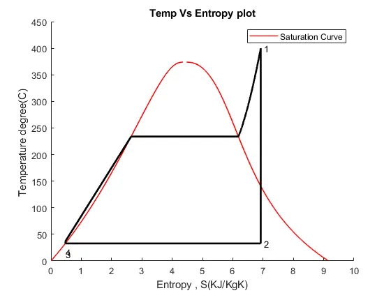
1.To create Rankine cycle simulator

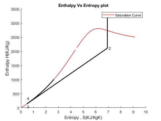
2.To plot T-s and h-s Diagram

MAIN BODY OF THE CONTENT :

1.Theory

• The Rankine cycle is an idealized thermodynamic cycle of a constant pressure heat engine that converts part of heat into mechanical work. In this cycle the heat is supplied externally to a closed loop, which usually uses water (in a liquid and vapor phase) as the working fluid.
• This cycle is composed of four key parts: the generation of high-pressure steam, a turbine, a condenser, and a pump.
• There are four processes in the Rankine cycle which are as follows:

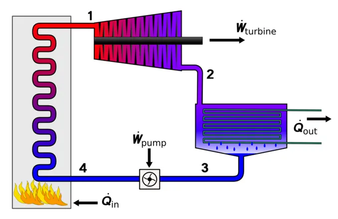
(i) 1-2 : Isentropic Expansion - The dry saturated vapour expands through a turbine , generating power. This decreases the temperature and pressure of the vapour, and some condensation may occur.

(ii) 2-3 : Constant pressure heat rejection - The wet vapour then enters a condeser , where it is condensed at a constant pressure to become a saturated liquid.

(iii) 3-4 : Isentropic Compression - The working fluid is pumped from low to high pressure. As the fluid is a liquid at this stage, the pump requires little input energy.

(iv) 4-1 : Constant pressure heat addition - The high-pressure liquid enters a boiler, where it is heated at constant pressure by an external heat source to become a dry saturated vapour.

2. Code

clear all
close all
clc
disp('                                                        RANKINE CYCLE')
fprintf('\n\n')
disp('1-2 is Isentropic expansion in the Turbine')
disp('2-3 is constant pressure Heat rejection by the condenser')
disp('3-4 is Isentropic compression in the pump')
disp('4-1 is constant pressure Heat addition by the boiler')

%Obtaining input from the user
fprintf('\n')
p1 = input('Enter the Pressure at the Turbine inlet ( in bar) : ');

T1 = input('Enter the Temperature at the Turbine inlet ( in Degree Celcius) : ');

p2 = input('Enter the Pressure at the condeser (in bar) : ');


%State 1
h1 = XSteam('h_pT', p1 , T1 );
s1 = XSteam('s_pT', p1 , T1);

%State2
s2 = s1;
sf2 = XSteam('sL_p' , p2);
sg2 = XSteam('sV_p' , p2);
x2 = (s2-sf2)/(sg2-sf2);
hf2 = XSteam('hL_p' , p2);
hg2 = XSteam('hV_p' , p2);
h2 = hf2 + (x2*(hg2-hf2));

%State3
p3 = p2;
s3 = XSteam('sL_p' , p3);
h3 = XSteam('hL_p' , p3);

%State4
s4 = s3;
p4 = p1;

%Work done by the Turbine
Wt = h1-h2;


%Work done on the Pump
v3=XSteam('vL_p' , p3);
Wp = v3*(p4-p3)*100
h4 = h3 + Wp;

%Back Work Ratio
Bw_Ratio = Wp/Wt;

%Net Work
Wnet = Wt - Wp;

%Heat into the system
Qin = h1 - h4;

%Heat Out of the system
Qout = h2 - h3;

%Thermal Efficiency
Eff = (Wnet/Qin)*100;

%Specific Steam Consumption
SSC = (3600/Wnet);

%Calculating Temperatures at the state poits
T3 = XSteam('Tsat_p' , p3);
T2=T3;
Cp4 = XSteam('Cp_ps',p4,s4);
Cv4 = XSteam('Cv_ps',p4,s4);
k = Cp4 / Cv4;
T4 = T3 / ((p3/p4)^((k-1)/k));


%Calculating Temperature , enthalpy and Entropy at the vapour and liquid
%line for plotting

T6 = XSteam('Tsat_p' , p1);
s5 = XSteam('sL_p' , p1);
s6 = XSteam('sV_p' , p1);
h5 = XSteam('hL_p' , p1);
h6 = XSteam('hV_p' , p1);
T5 = T6;
%Plotting the saturation Curve
T = linspace(1,375,1000);
for i=1:length(T);
sf(i) = XSteam('sL_T' , T(i));
sg(i) = XSteam('sV_T' , T(i));
hf(i) = XSteam('hL_T' , T(i));
hg(i) = XSteam('hV_T' , T(i));
end

%Plotting T-s Diagram
figure(1)
hold on
plot(sf , T , 'r' , 'linewidth' , 1)
plot(sg , T , 'r' , 'linewidth' , 1)
plot([s1 s2] , [T1 T2] , 'k' , 'linewidth' , 2);
plot([s2 s3] , [T2 T3] , 'k' , 'linewidth' , 2);
plot([s3 s4] , [T3 T4] , 'k' , 'linewidth' , 2);
plot([s4 s5] , [T4 T5] , 'k' , 'linewidth' , 2);
plot([s5 s6] , [T5 T6] , 'k' , 'linewidth' , 2);
sc1 = linspace(s6 , s1 , 1000);
for j=1:length(sc1);
    Tc1(j) = XSteam('T_ps' , p1 , sc1(j));
end
plot(sc1 , Tc1 , 'k' , 'linewidth' , 2)
text(s1+0.1,T1,'1')
text(s2+0.1,T2,'2')
text(s3 , T3-20 , '3')
text(s4 , T4-20 , '4')
title('Temp Vs Entropy plot')
xlabel('Entropy , S(KJ/KgK)')
ylabel('Temperature degree(C) ');
legend('Saturation Curve')

%Plotting h-s Curve
figure(2)
hold on
plot(sf , hf , 'r' , 'linewidth' , 1)
plot(sg , hg , 'r' , 'linewidth' , 1)
plot([s1 s2] , [h1 h2] , 'k' , 'linewidth' , 2);
plot([s2 s3] , [h2 h3] , 'k' , 'linewidth' , 2);
plot([s3 s4] , [h3 h4] , 'k' , 'linewidth' , 2);
hc = linspace(h4 , h5 , 100);
for k=1:length(hc);
    sch(k) = XSteam('s_ph' , p1 , hc(k));
end
plot(sch , hc , 'k' , 'linewidth' , 2)
text(s1+0.1,h1,'1')
text(s2+0.1,h2,'2')
text(s3 , h3-100 , '3')
text(s4 , h4+200 , '4')
title('Enthalpy Vs Entropy plot')
xlabel('Entropy , S(KJ/KgK)')
ylabel('Enthalpy H(KJ/Kg)');
legend('Saturation Curve')

%Displaying Results
disp('RESULTS');
fprintf('\n');
fprintf('At state point 1');
fprintf('\n');
fprintf('p1:%8.3f bar' , p1);
fprintf('\n');
fprintf('T1:%8.3f degree celcius' , T1);
fprintf('\n');
fprintf('h1:%8.3f KJ/Kg' , h1);
fprintf('\n');
fprintf('s1:%8.3f KJ/KgK' , s1);
fprintf('\n');
fprintf('\n');

fprintf('At state point 2');
fprintf('\n');
fprintf('p2:%8.3f bar' , p2);
fprintf('\n');
fprintf('T2:%8.3f Degree Celcius' , T2);
fprintf('\n');
fprintf('h2:%8.3f KJ/Kg' , h2);
fprintf('\n');
fprintf('s2:%8.3f KJ/KgK' , s2);
fprintf('\n');
fprintf('x2:%8.3fnn' , x2);
fprintf('\n');
fprintf('\n');

fprintf('At state point 3');
fprintf('\n');
fprintf('p3:%8.3f bar' , p3);
fprintf('\n');
fprintf('T3:%8.3f Degree Celcius' , T3);
fprintf('\n');
fprintf('h3:%8.3f KJ/Kg' , h3);
fprintf('\n');
fprintf('s3:%8.3f KJ/KgK' , s3);
fprintf('\n');
fprintf('\n');

fprintf('At state point 4');
fprintf('\n');
fprintf('p4:%8.3f bar' , p4);
fprintf('\n');
fprintf('T4:%8.3f Degree Celcius' , T4);
fprintf('\n');
fprintf('h4:%8.3f KJ/Kg' , h4);
fprintf('\n');
fprintf('s4:%8.3f KJ/KgK' , s4);
fprintf('\n');
fprintf('\n');

fprintf('Turbine work:%8.3f KJ/Kg' , Wt);
fprintf('\n');
fprintf('Pump work:%8.3f KJ/Kg' , Wp);
fprintf('\n');
fprintf('Net Work Output:%8.3f KJ/Kg' , Wnet);
fprintf('\n');
fprintf('Back Work Ratio:%8.3f ' , Bw_Ratio);
fprintf('\n');
fprintf('Efficiency:%8.3f percent ' , Eff);
fprintf('\n');
fprintf('S.C.C:%8.3f KJ/Kwh' ,SSC );
fprintf('\n');


    

3.Explanation of code

• Clear all , close all , clc are used to clear the workspace , close all figures and clear the command window respectively.
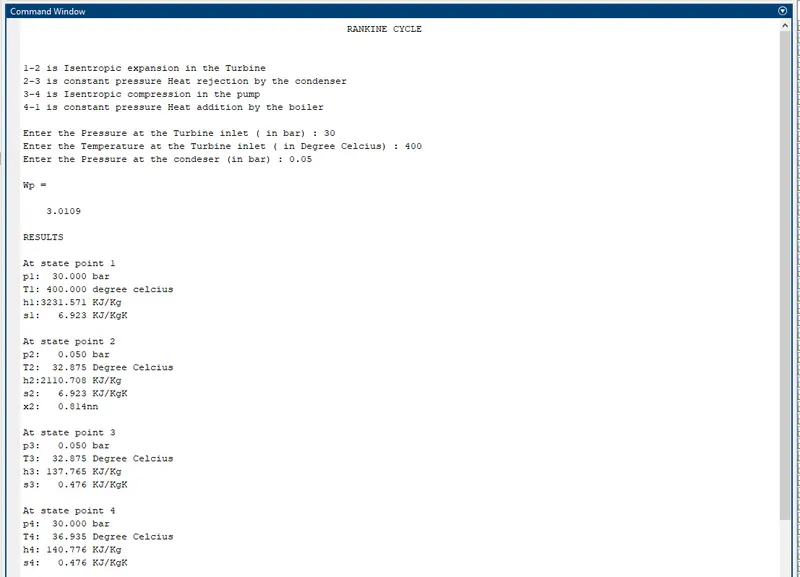
• Using disp command name of the project ('RANKINE CYCLE') is displayed.Similarly, processes taking place in the rankine cycle are also displayed.
• input command will ask user to enter the inlet pressure , inlet temperature at turbine and pressure at condenser which is stored inside the variables p1 , T1 and p2 respectively.
• XSteam file contains values of steam and water properties such as Enthaply, Entropy etc. at specific Temperature and pressure. Using this file we have extracted the values at all the states. In between some thermodynamic relations(formulaes) has been used to find out the properties sequentially. e.g.XSteam('h_pT', p1 , T1 ) which will retuen enthalpy value for given pressure p1 and temperature T1.
• Using Rankine cycle formules , work done of pump , turbine , net work , back work ratio and thermodynamic efficiency is calculated.
• Next set of code is implemented to calculate temperature values at all the states.
• Then for plotting saturation curve array of 1000 temperature values is used starting from 1 to 375. By the use of for loop at each value of temperature from xsteam table it will plot the saturation curve .
• Using plot command all the state points are plotted and joined with line.
• from sg to point 1 the plot is curve hence we used array which will take 1000 values of temperature and entropy to create smooth curve.
• Using text command numbering of state point is done with suitable offset so that numbers won't overlapped.
• Similarly h-s curve is plot.
• Finally, all the results are plotted using printf command.

4.Results

5. T-s Diagram

6. h-s Diagram